MATH3401 — Complex Analysis

Lecture 1 — The Complex Field

Joseph Grotowski: [email protected]. 06-206 (Tues 10-12, Thurs 11-12, or by appointment).

Introduction

This course is compulsory for many students. Its prerequisites are MATH2000 and MATH2400 (or equivalents). This is the capstone course for math majors and math undergraduate degrees.

The techniques and problem solving strategies in this course will be beneficial in many ways.

Lecture recordings will be on the Blackboard. Tutorials start in week 1.

Assessment

The best 5 of 6 assignments together count for 20%. The midsemester counts for 20% (one page of handwritten notes is allowed, single-sided). The final exam counts for 60% (one page of handwritten notes, double-sided).

Complex analysis

Cool stuff

A ‘nice’ result which shows all different parts of maths coming together: e^{i\pi} = -1.

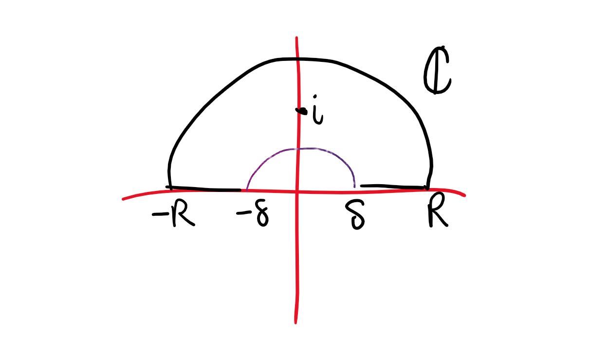
There are a number of fascinating things about this equation. Despite i not appearing in this expression, it still delves into complex analysis. \int_{0}^\infty \frac {\sin x} x \,dx = \frac \pi 2 A reasonable question is does this integral even converge? If we replace \sin x with 1, the integral diverges by the p-test. Arguing the integral exists is a bad time without complex analysis, but is really really nice with complex. This will be done towards the end of the semester, making use of contour integrals around a path in the complex plane.

In the more applied realm, we can also do things with fluid flow. A very expensive method would be constructing a physical model then running experiments. 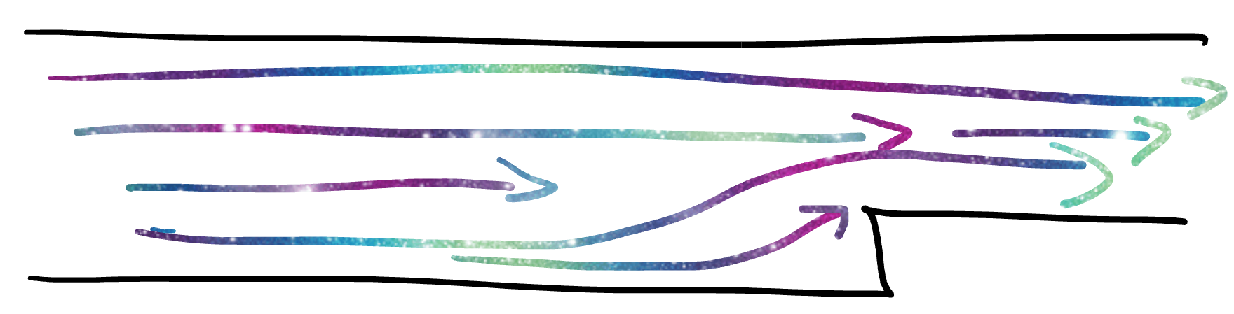With complex analysis, we can perform analysis on a straight pipe, then map to the pipe above without having to build the channel. We can just tweak the parameters in the map to test different scenarios. This is called a conformal transoformation.

Similarly, Joukowski transformations can be used to model air flow around a wing.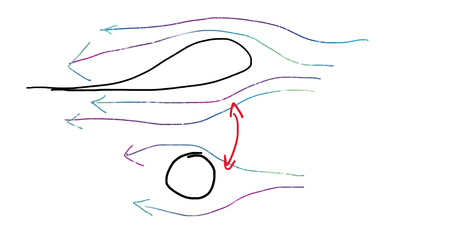

We can also get nice results about series like \begin{aligned} \frac 1 {1^2} + \frac 1{2^2} + \frac1 {3^2} + \cdots &= \frac {\pi^2} 6 \\ \frac 1 {1^2} - \frac 1{2^2} + \frac1 {3^2} - \frac 1 {4^2} +\cdots &= \frac {\pi^2} {12} \\ \sum_{k=1}^\infty \frac 1 {1 + 4 k^2 \pi^2}& = \frac 1 2 \left(\frac 1 {e-1} - \frac 1 2\right) \end{aligned}

Riemann Zeta

\zeta (s) = \sum_{n=1}^\infty \frac 1 {n^s} = \prod_{p\ \text{prime}}(1-p^{-s})^{-1} (The product of primes result is from Euler. This is called the Riemann zeta function)

Riemann hypothesis: \zeta has infinitely many non-trivial zeros and they all lie on the line \text{Re}(s) = 1/2.

Note that the expression for \zeta only makes sense for \text{Re} s) > 1, so we need to extend it to \mathbb C via analytic continuation. In doing this, the trivial zeros are -2, -4, -6, \dots

Lecture 2 — Complex Numbers

\renewcommand\Re{\operatorname{Re}} \renewcommand\Im{\operatorname{Im}}

Complex numbers have been around for a while.

• In 1545, Cardano looked at real roots of x^3 + ax + b. He found 5 + \sqrt{-15} and called it “mental torture”.
• In 1575, the algebraic rules for i were first described.
• In 1629, a+\sqrt{-b} was called “solutions impossibles” by Girard.
• In 1637, Descartes discovered imaginary numbers.
• From 1831 onwards, complex numbers.

\mathbb C as a field

B.C section 1-3

\begin{aligned} \mathbb N &= \{1, 2, 3, \ldots \} \\ \mathbb N_0 &= \{0, 1, 2, 3, \ldots \} \\ \mathbb Z &= \{0, \pm1, \pm2, \pm3, \ldots \} \\ \mathbb Q &= \{p/q : p, q \in \mathbb Z, q \ne 0 \} \\ \mathbb R &= \text{real numbers} \\ \mathbb C &= \text{complex numbers} \end{aligned}

Note that \mathbb Q is actually equivalence classes of “quotients” of integers because certain expressions are equivalent (see MATH2401). \mathbb R can be defined in several technical ways, such as Dedekind cuts or limits of sequences.

\mathbb C can be represented in various (equivalent) ways:

• z = (x, y) \in \mathbb C, for x, y \in \mathbb R. This is the “complex plane”. Alternatively, z = x(1, 0) + y(0, 1).
• z = x + ij, where x = \operatorname{Re}(z) and y = \operatorname{Im}(z).

i is the complex number represented by (0,1). We say \mathbb R \subset \mathbb C by identifying the complex number x + 0i with the real number x.

Addition in \mathbb C

\begin{aligned} (x_1, y_1) + (x_2, y_2) &= (x_1 + x_2, y_1 + y_2) \\ (x_1 + iy_1) + (x_2 + iy_2) &= (x_1 + x_2) + i(y_1 + y_2) \end{aligned}

Multiplication in \mathbb C

Denoted by \times or \cdot or juxtaposition (that is, putting things next to each other). \begin{aligned} (x_1, y_1)\cdot(x_2, y_2) &= (x_1x_2 - y_1y_2, y_1x_2 + x_1y_2) \\ (x_1 + iy_1) \cdot (x_2 + iy_2) &= (x_1 x_2 - y_1y_2) + i(y_1x_2 + x_1y_2) \end{aligned} The definition of multiplication formally applies if we use the usual rules for algebra in \mathbb R and set i^2 = -1.

Note: Multiplication of two complex numbers sums their angles (where positive is CCW) and multiples their radius.

\mathbb C is a field

With this addition and multiplication, \mathbb C is a field. Check: \mathbb C must be closed under the binary operations + and \cdot.

F2: + has identity 0+0i and inverse (-x) + i(-y). F5: \cdot has identity 1 + 0i and inverse z^{-1} = 1/(x+iy) \cdot (x-iy)/(x-iy) = \frac x{x^2+y^2} - i\frac{y}{x^2+y^2}

Since \mathbb C is a field, it holds: z_1, z_2 = 0 \implies z_1 = 0 \text{ or }z_2 = 0. This is the null-factor law and holds because on all fields. Also, we have (z_1z_2)^{-1} = z_1^{-1}z_2^{-1}.

Note: i^2 = -1 and (-i)^2 = -1. These are the only two solutions of z^2 = -1 in the complex numbers (we cannot check this yet). This is due to the Fundamental Theorem of Algebra.

Remark: \mathbb C is not ordered and, in fact, cannot be ordered. Thus, i is no more special then -i.

B.C. 4, 5

Given z = x + iy \in \mathbb C, there are a few useful functions to have: - modulus: |\cdot| : \mathbb C \to \mathbb [0, \infty), where |z| = \sqrt{x^2 + y^2}, - real part: \operatorname{Re}(z) = x, imaginary part: \operatorname{Im}(z) = y (both \mathbb C \to \mathbb R),

Lecture 3 — Functions of Complex Numbers

Complex conjugate

The complex conjugate is defined as a function \bar \cdot : \Complex \to \Complex, where (x + iy) \mapsto (x - iy). Geometrically, this reflects a complex number about the real axis.

Properties

\begin{aligned} z = \bar z \iff \operatorname{Im}(z)&= 0 \text{ (i.e. z} \in \mathbb R \text{)} \\ \overline {(\bar z)} &= z \\ \overline {zw} &= \bar z \bar w \\ \overline{z+w} &= \bar z + \bar w \\ \overline {z^{-1}} &= (\bar z)^{-1}, z \ne 0 \\ |z|^2 &= z \bar z \\ \operatorname{Re}(z) &= \frac{z + \bar z} 2 \\ \operatorname{Im}(z) &= \frac{z - \bar z} 2 \end{aligned}

A very useful property (from MATH1051) is the triangle inequality: |z+w| \le |z| + |w|. 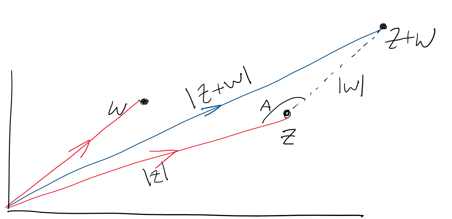Proof: More specifically using the cosine rule, |z+w|^2 = |z|^2 + |w|^2 - 2|z||w|\cos A. This is a true and exact statement. However, in analysis, we often want to make these statements less precise but more useful. Because -1 \le \cos \le 1, \begin{aligned} |z+w|^2 &\le |z|^2 + |w|^2 + 2|z||w| \\ &= (|z| + |w|)^2\\ \implies |z+w| &\le |z| + |w| \end{aligned}

Polar coordinates

B.C. 6-9

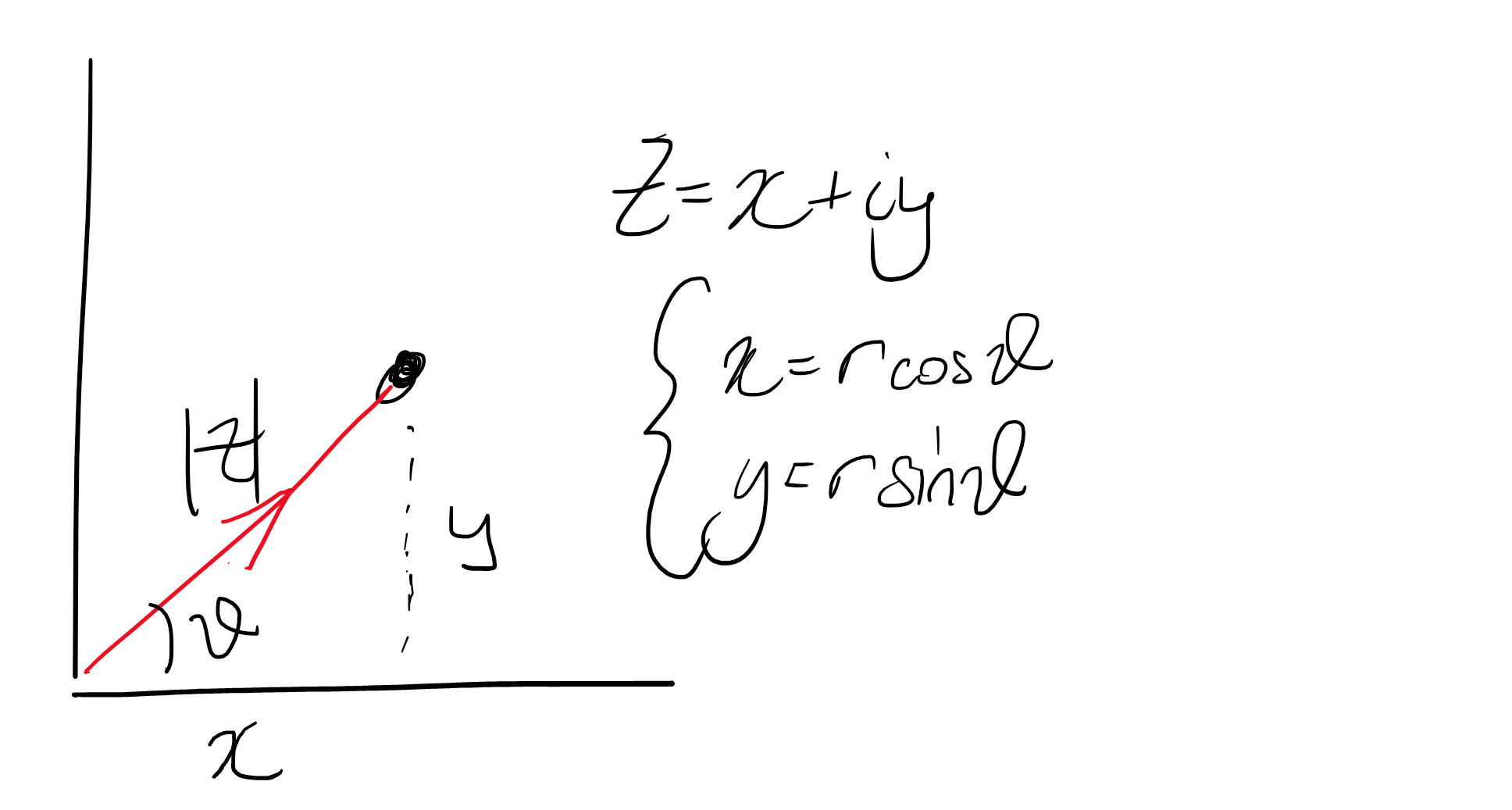
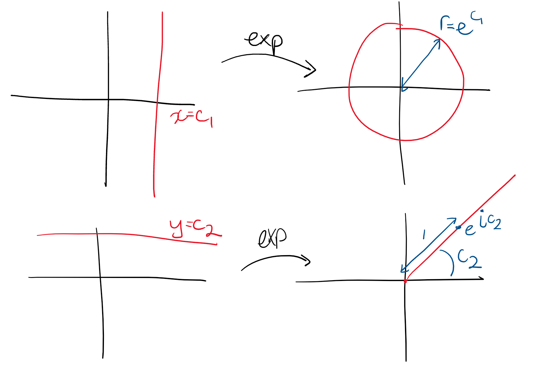
Given a complex number z = x+iy, we can find r and \theta such that x = r \cos \theta, \text{ and }\ y = r \sin \theta. Then, we can also write it using Euler’s formula (as a formal convention for the moment): z = re^{i\theta} = r(\cos \theta + i \sin \theta). Remark: this formula follows formally from the Taylor series of e^{i\theta}.

Here, \theta is an (as opposed to the) argument of the complex number z. We write \theta = \arg z. Here, \arg is not a (single-valued) function. Given a \theta, we can always take \theta + 2\pi which will satisfy the x and y equations. Also, for z=0, any \theta will work.

To make \arg a function, we need to restrict its range. There are two options: 0 to 2 \pi and -\pi to \pi. In complex analysis, we normally use the second. Specifically, \operatorname{Arg} z is defined to be the unique values of \theta such that -\pi < \arg z \le \pi.

Examples: - \operatorname{Arg}(1+i) = \pi / 4 but \arg (1+i) = \ldots, -7\pi/4, \pi/4, 9\pi/4, \ldots. - \operatorname{Arg}(-1) = \pi. - \operatorname{Arg}(0) is undefined, but \arg (0) = \mathbb R.

In summary, \operatorname{Arg} is a function \mathbb C \setminus \{0\} \to (-\pi, \pi]. Alternative notation for \mathbb C \setminus \{0\} is \mathbb C^* or \mathbb C_*.

Note: \begin{aligned} |e^{i\theta}| &= 1 \text{ (easy to check)}\\ (e^{i\theta})^{-1} = e^{-i\theta} &= \overline {e^{i\theta}} \\ (re^{i\theta})(\rho e^{i\phi}) &= (r\rho) e^{i(\theta + \phi)} \\ \implies |zw| &= |z| |w|,\enspace \arg (zw) + \arg z \arg w \end{aligned} However, the last equality does not necessarily hold for \operatorname{Arg}. For example, with z = w = {(-1 + i)/\sqrt 2}

De Moivre’s formula

z = re^{i\theta} \implies z^n = r^n e^{in\theta}, \quad n \in \mathbb Z. In particular, e^{in\theta} = (\cos \theta + i \sin \theta)^n = \cos(n\theta) + i \sin (n\theta).

Lecture 4 — Functions as Mappings

Roots of a complex number

What is the number z such that z^n gives us the original number? By the fundamental theorem of algebra, we know there ar exactly n n-th roots in \mathbb C.

Consider the n-th roots of z = re^{i\theta}, for z \in \mathbb C_*. That is, we want all w \in \mathbb C such that w^n = z. Notation: \exp (\xi) = e^\xi.

Then, we can use de Moivre’s theorem “in reverse” to see that z has n distinct roots: \left\{ r^{1/n}\exp\left(\frac{i\theta}n\right), r^{1/n}\exp\left(\frac{i\theta}n + \frac{i2\pi}n\right), \ldots, r^{1/n}\exp\left(\frac{i\theta}n + \frac{i2\pi(n-1)}n\right) \right\}

B.C. 13 (8th ed 12-13)

Functions & mappings

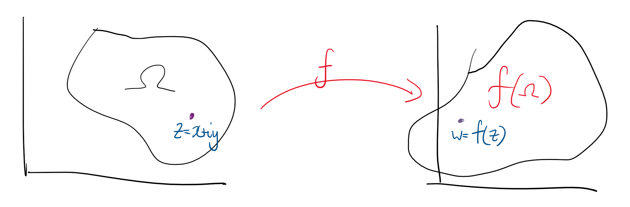
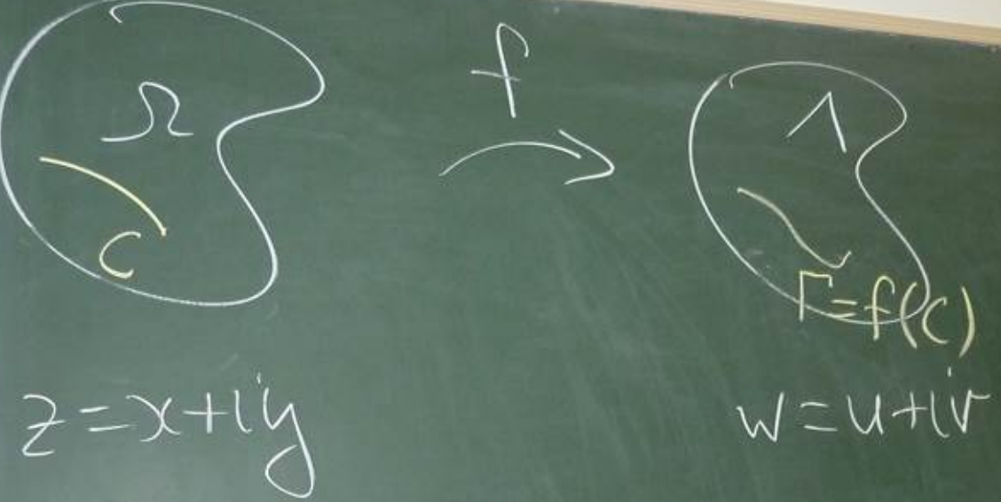
Suppose we have \Omega \subseteq \mathbb C and a function f : \Omega \to \mathbb C can be viewed as a mapping on \Omega, the domain of f. If \Omega is not specified, then we take \Omega to be as large as possible.

Example: For f(z) = 1/z we can take \Omega = \mathbb C \setminus\{0\}, so f : \mathbb C_* \to \mathbb C. As notation, we can also write f : z \mapsto 1/x, or w=1/z, or just 1/z if the meaning is clear.

The usual notation is w : (x,y) \mapsto (u,v), i.e. w(x+iy)=u(x+iy)+iv(x+iy) or w(x,y)=u(x,y)+iv(x,y).

This notation is not completely rigorous; u is both a function from \mathbb C and from \mathbb R^2. We could introduce a map \varphi : (x,y)\mapsto (x+iy) but this is excessively verbose. There is no real problem with this, but be aware.

Definitions

• The domain of f is \Omega, also denoted \operatorname{dom} f.
• The range of f is f(\Omega) = \operatorname{Range}f=\{w : w = f(z) \text{ for some }z \in \Omega\}.
• The inverse of f is f^{-1}(\xi) = \{z \in \Omega : f(z) = \xi\}. Note that this returns sets. If there is only one element, we can just call that element the “inverse”.

Examples: - Consider f(z) = 1/z. \operatorname{dom}f = \mathbb C_\star. f^{-1}(\xi)=1/z is a function \mathbb C_* \to \mathbb C_*. - For g(z) = 1/(1-|z|^2). \operatorname{dom}g = \mathbb C \setminus \{z : |z| = 1\}. The function is g : \{z : z \ne 1\} \to \mathbb R. The inverse is not a function. - For h(z) = z^n where h : \mathbb C \to \mathbb C, the inverse is also not a function.

Geometric intuition

Let’s aim to get a geometric picture of what a given f does.

Examples: - w = 1+z moves each point one unit to the right (in the positive real direction). - re^{i\theta} \mapsto re^{i(\theta+\pi/2)} rotates points through an angle of \pi/2 in the counter-clockwise direction about the origin.

For new and unfamiliar mappings, break them down into compositions of known or easy maps.

Examples: - w = Az + b where A, b \in \mathbb C and A \ne 0. We can think of A as a dilation and rotation, then +b as a translation. - For z \mapsto Az, write A=a e^{i\alpha} for \alpha, a \in \mathbb R. This gives us re^{i\theta}\mapsto ar e^{i(\theta+\alpha)}. Specifically, it dilates the modulus by a factor of a=|A| and rotates through \alpha = \arg A. - For z \mapsto z+b where b = b_1+b_2i, b_1, b_2 \in \mathbb R. This translates b_1 to the right and b_2 up. If negative, goes in the opposite direction.

Note: The maps above have domain and image \mathbb C.

Lecture 5 — Mappings 2

Another very important map to look at is z \mapsto 1/z on \mathbb C_*. We can write this as the composition of two slightly more complicated functions.

Define \xi(z) = z/|z|^2 on \mathbb C_* and \eta(z) = \bar z. For z \in \mathbb C_*, we can compose these two as \begin{aligned} \eta \circ \xi(z) = \eta(\xi(z)) = \overline {\left(\frac z {|z|^2}\right)} = \frac{\bar z}{|z|^2} = \frac {\bar z}{z \bar z} = \frac 1 z. \end{aligned}

\xi is called inversion, with respect to the unit circle. \eta is just reflection about the real axis.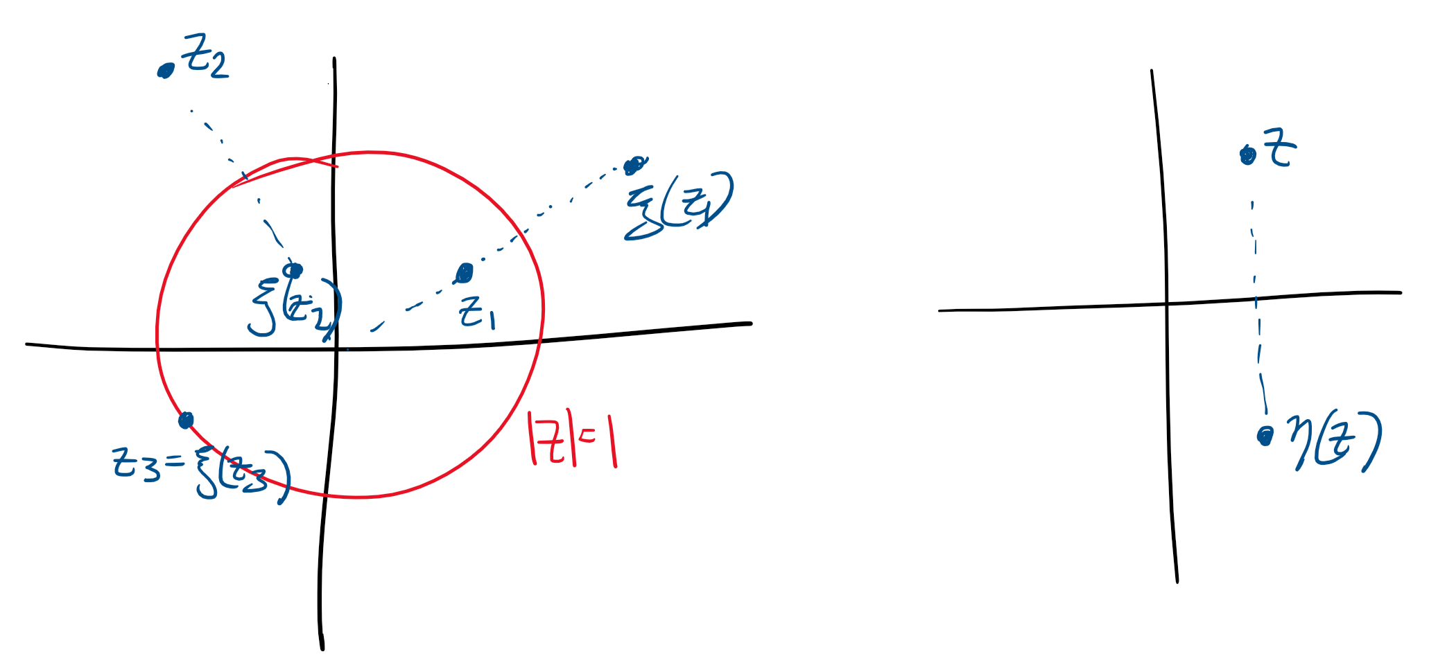

For w = 1/z = \bar z / |z|^2 we can write it as x+iy \mapsto u+iv, where w=\frac{x-iy}{x^2 + y^2} \quad\implies\quad u = \frac{x}{x^2+y^2}, \quad v=\frac{-y}{x^2+y^2}. We can use this to show the following statement: 1/z maps circles and lines in the z=plane to circles and lines in the w-plane. Note that this does not require circles to map to circles, or lines to map to lines.

The key point is both circles and lines in the z-plane can be represented as A(x^2+y^2)+Bx+Cy+D=0,\quad\text{ where } B^2+C^2 > 4AD for A,B,C,D \in \mathbb R. If A=0, then the equation is a circle. The inequality constraint tells us that \begin{aligned} \left(x+\frac B {2A}\right)^2 + \left(y+\frac C {2A}\right)^2 = \left(\frac{\sqrt{B^2+C^2-4AD}}{2A}\right)^2. \end{aligned} Note, for w = 1/z, the u and v expressions earlier tell us that w has the form D(u^2+v^2)+Bu-Cv+A=0 which is a circle or line.

Terminology

• f : \Omega \to \mathbb C is 1-to-1 or injective if f(z) = f(\xi) implies z = \xi.
• f : \Omega \to \Lambda, where \Lambda \subseteq \mathbb C, is onto or surjective if for all \eta \in \Lambda, there exists (one or more) z \in \Omega such that f(z) = \eta.

Examples: Affine transformations are bijections \mathbb C \to\mathbb C , and 1/z is a binection \mathbb C_* \to \mathbb C_*.

Möbius transformations

B.C. 99 (8th ed 93)

Let a, b, c, d \in \mathbb C where ad-bc \ne 0. Then, w = T(z) = \frac{az+b}{cz+d} is called a Möbius (or linear fractional) transformation. The natural domain of definition is - if c = 0, then \operatorname{dom}w = \mathbb C (because c = 0\implies d \ne 0), or - if c \ne 0, then \operatorname{dom}w = \mathbb C \setminus \{-d/c\}.

Let’s try to understand T geometrically.

Claim: T is injective and surjective from \mathbb C \to \mathbb C. Proof. For c = 0, then to prove injectiveness suppose T(z) = T(\xi). We want to show z = \xi. Substituting into the formula for T, \frac a d z + \frac b d = \frac a d \xi + \frac b d \implies z = \xi. To prove it is surjective, given w \in \mathbb C, we need z \in \mathbb C such that T(z) = w. The value z = d/a(w-b/d) satisfies this.

For c \ne 0, consider \begin{aligned} w &= \frac{az+b}{cz+d} = \frac{a(z+d/c) - ad/c + b}{c(z+d/c)}\\ &= \frac a c + \left(\frac{bc-ad}c\right)\frac 1 {cz-d} \end{aligned} This is a composition of a linear transformation, 1/z and another linear transformation.

Thus, T is the composition of linear and 1/z maps. That is, Z_1 = cz+d, \quad W = 1/Z_1, \quad w = \frac a z + \frac{bc-ad}cW. In both cases, Möbius transformations are compositions of maps previously studied. This means they are bijective.

Lecture 6 — Möbius Transformations 2 & The Extended Complex Plane

Recall that T(z) = w = \frac{az+b}{cz+d} (ad-bc \ne 0) is a Möbius transformation.

It can be rewritten as Azw + Bz + Cw + D = 0 where A = c, B = -a, C=d, D=b. This is called the implicit form.

Recall that case 1 was c = 0, which reduces T to a linear transformation which is a bijection \mathbb C \to \mathbb C. Case 2 was also a bijection from \mathbb C \setminus \{-d/c\} \to \mathbb C \setminus \{a/c\}, with inverse T^{-1}(w) = \frac{-dw+b}{cw-a}.

A question might be can we extend T to a function \mathbb C \to \mathbb C in case 2? In particular, such that the extension is injective and surjective. The answer is yes, by “plugging the hole”. We simply define T(-d/c) = a/c. However, this is unsatisfying because the function becomes discontinuous.

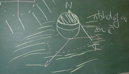
An important concept: We are going to extend \mathbb C to the extended complex plane, written \bar{ \mathbb C}. This is done by adding a point at infinity, which is called \infty. We can think of the complex plane as a sphere with the origin at one pole and this \infty at the other, with distances expanding as you go further from 0.

We then define T(-d/c) = \infty and T(\infty) = a/c. This extends T to a map \bar {\mathbb C }\to \bar {\mathbb C} which is injective and surjective.

Remark: \bar {\mathbb C} is a topological space and the above extension is continuous. A topology on a set is a space with so-called “open sets”. Intuitively, points can be ‘nearby’ to other points.

\bar {\mathbb C} can be visualised as the Riemann sphere. The origin 0+0i is at the south pole. A point on the complex plane is mapped uniquely to a point on the sphere. This is done by picking the point on the sphere’s surface on the line between the point and the north pole. “Infinity” can be thought of as the north pole.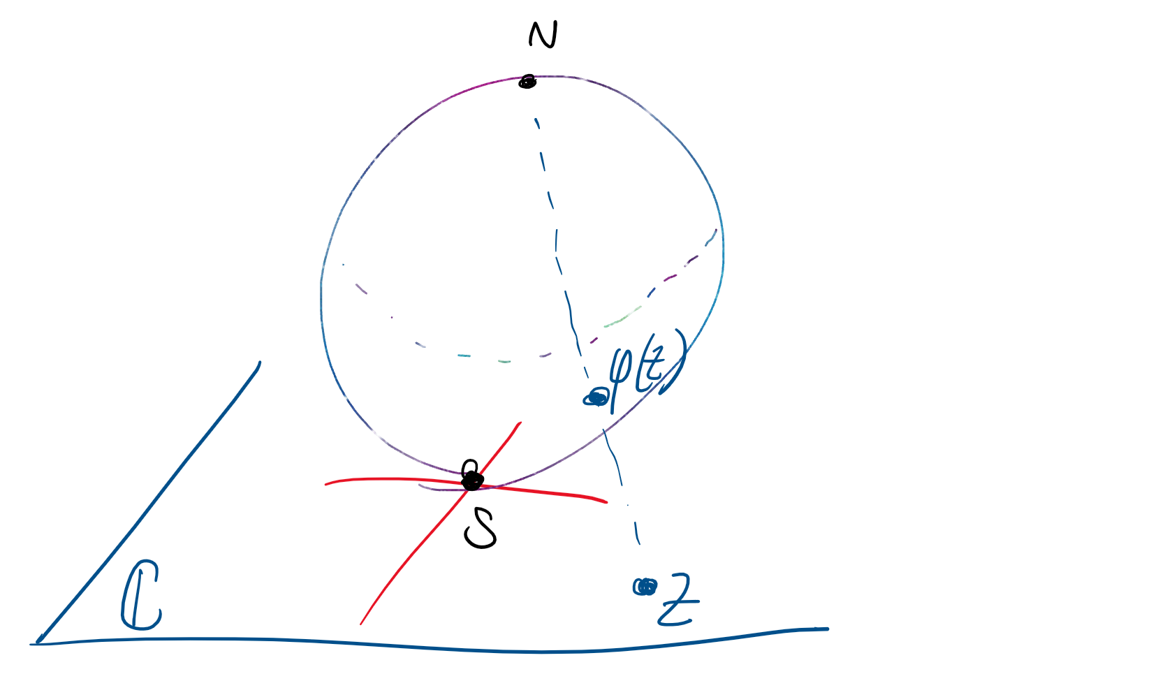

A few final remarks on Möbius transformations. Given 3 distinct points in z_1, z_2, z_3\in\bar{ \mathbb C} and 3 different distinct points w_1, w_2, w_3 \in \bar {\mathbb C}, there exists a unique Möbius transformation T such that T(z_1) = w_1, \ T(z_2)=w_2, \text{ and }T(z_3)=w_3. In fact, T is given by \frac{(w-w_1)(w_2-w_3)}{(w-w_3)(w_2-w_1)} = \frac{(z-z_1)(z_2-z_3)}{(z-z_3)(z_2-z_1)}. In practice, it may be easier to directly solve for a,b,c,d than using the above expression.

Note: How does this work with infinity? \begin{aligned} T(\infty) = a/c &\iff \lim_{|z|\to\infty} T(z) = a/c\\ T(-d/c) = \infty &\iff \lim_{z\to -d/c} 1/T(z) = 0 \end{aligned}

Lecture 7 — Exponential Maps

A note on coronavirus about the recent mail from Joanne Wright, the DVC(A).

Recall the Möbius transformation, and note that is is unique up to scaling for \lambda > 0. w = \frac{az+b}{cz+d} = \frac{\lambda az+\lambda b}{\lambda cz+\lambda d}

Remark: Any map from the inside of a (upper half) half-plane to the inside of a circle has the form w = e^{-i\alpha} \frac{z-z_0}{z-z_0}\quad \text{ for some }\alpha \in \mathbb R, z_0 \in \mathbb C, \operatorname{Im} z_0 > 0.

Exponential map

B.C. 103 (8Ed 104)

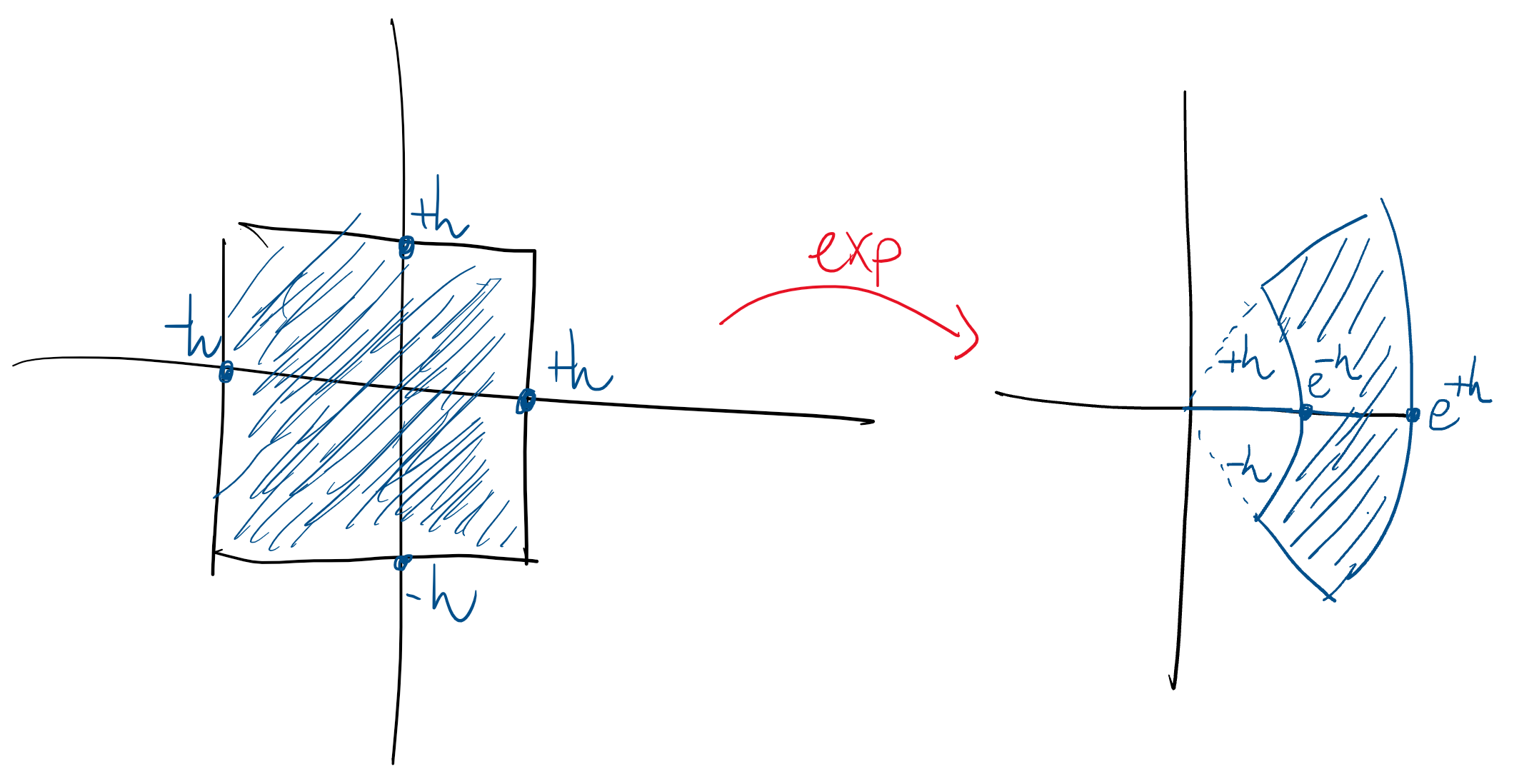
z \mapsto e^z = \exp x = w, \quad \operatorname{dom} w = \mathbb C. Given a z = x+iy for x, y \in \mathbb R, w = e^z = e^{x+iy} = e^x e^{iy} = e^x (\cos y + i \sin y) = u+iv\\[0.7em] \begin{aligned} \text{ where }\quad u &= e^x \cos y\\ v &= e^x \sin y. \end{aligned} This is easier to see by writing w = \rho e^{i\phi} where \rho = e^x, \phi = y + 2k\pi for k \in \mathbb Z. This function is periodic in \mathbb C.

Images under exp

Properties

Many of the properties of the real \exp extend to \mathbb C. Such as - e^0 = 1. - e^{-z} = 1/e^z. - e^{z_1+z_2} = e^{z_1}e^{z_2}. - e^{z_1-z_2} = e^{z_1}/e^{z_2}. - (e^{z_1})^{z_2} = e^{z_1z_2}.

However, some things do not extend: - e^x > 0~\forall x \in \mathbb R but, for example, e^{i\phi} = -1. - x \mapsto e^x is monotone increasing for x \in \mathbb R but z \mapsto e^z is periodic with period 2\pi i.

Note: As in \mathbb R, e^z = 0 has no solution in \mathbb C. If there was some z = x+iy such that e^z = 0, then e^x e^{iy} = 0 \implies e^x = 0 because |e^{iy}| = 1, contradiction.

Inverses

B.C. 31-33 (8Ed 30-32)

We have a function f : \Omega \to \mathbb C. Then, g : \operatorname{Range}f \to \Omega is an inverse of f if g \circ f : \Omega \to \Omega is the identity. That is, (g \circ f)(z) = z for all z \in \Omega.

Example: z \mapsto z+1 and z \mapsto z-1 are inverses for \mathbb C \to \mathbb C. z \mapsto 1/z is its own inverse \mathbb C_* \to \mathbb C_*.

Lecture 8 — Logarithm

Inverse of the exponential

The inverse of the exponential! It’s probably too much to hope for \log = \log_e to be the inverse, because \exp is periodic (with period 2\pi i) in \mathbb C.

Begin with e^w = z. Write z = re^{i\Theta}, r > 0, where \Theta = \operatorname{Arg} z \in (-\pi, \pi].

We can make our calculations clearer by using polar coordinates in the domain and rectangular coordinates in the range. That is, w = u+iv \implies z=e^w = e^{u+iv}=e^ue^{iv}\\ \implies e^u = r,\quad v=\Theta + 2k\pi, \quad k \in \mathbb Z. So u = \ln r, which (notation in this course) means logarithm with base e of the positive real number r. Thus, \begin{aligned} w &= u+iv \\ &= \ln r + i(\Theta + 2k\pi) \quad k \in \mathbb Z \\ &= \ln |z| + i \arg z \end{aligned} This defines the multi-valued function \log : \mathbb C_* \to \mathbb C_*. \begin{aligned} \exp (\log z) &= z\\ \log(\exp z) &= z + 2k\pi i \end{aligned} We can check the the properties of \log translate into \mathbb C. For example, (note that this is a statement of multi-valued functions) - \log (z\xi) = \log z + \log \xi. - \log (z / \xi) = \log z - \log \xi.

As with \operatorname{Arg} and \arg, we can define the principal logarithm, denoted \operatorname{Log} : \mathbb C_* \to \mathbb C_*, as \operatorname{Log} z = \ln |z| + i \operatorname{Arg} z This function is single-valued but has the disadvantage of being discontinuous on the negative real axis and 0, since \operatorname{Arg} is discontinuous there. Indeed, \operatorname{Log} and \operatorname{Arg} are not even defined at 0.

As with \operatorname{Arg}, it may be the case that \operatorname{Log}(z_1 z_2) \ne \operatorname{Log} z_1 + \operatorname{Log} z_2.

Complex exponents

Remark: In reals, we could define dsomething like 2^{\sqrt 2} as \lim_{n\to\infty}2^{a_n} where \{a_n\}\to\sqrt 2. This doesn’t quite work in complex.

Set z^c = \exp(c \log z). Because \log is multi-valued, this may result in a sequence of outputs. For c \in \mathbb N and 1/c \in \mathbb Z, we recover the formulas from the fourth lecture.

Remark: B.C. defines z^{1/n} as a multi-valued function and defines the principal value as \operatorname{PV}(z^{1/n}) = |z|^{1/n}\exp (i\operatorname{Arg} z / n). Similarly for z \mapsto z^c, \operatorname{PV}(z^{c}) = \exp(c \operatorname{Log} z) = \exp (c \ln |z| + ic \operatorname{Arg}a).

Example: As a concrete example, doable but easy to make mistakes, \begin{aligned} \operatorname{PV}[(1-i)^{4i}] &= \exp(4i (\ln |1-i| + i\operatorname{Arg}(1-i)))\\ &= \exp (4i \ln \sqrt 2 -4(-\pi/4))\\ &= e^{\pi}\exp(4i\ln \sqrt 2) \\ &= e^\pi (\cos(2\ln 2) + i\sin (2\ln 2)) \end{aligned}

Sometimes, we need to use a different single-valued \operatorname{Log} or \operatorname{Arg}. For example, if we need to integrate around a contour excluding the -i axis. In this case, we would define \operatorname{\mathcal {Arg}} z such that -\pi/2 < \arg z \le 3\pi/2. This leads to an alternative single-valued \mathcal {Log} and derived functions.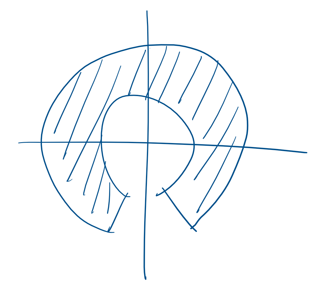

Next: square roots, branch cuts.

Lecture 9 — Branch Cuts & Trigonometric Functions

B-C 108.

A branch is a half-open interval of the form \alpha \le \theta < \alpha + 2\pi or \alpha < \tilde \theta \le \alpha + 2\pi of \mathbb R.

This is good because we can define a single-valued \operatorname{Arg} with values in this interval, a single-valued \operatorname{Log}, as well as a single-valued branch of, for example, z^{1/2}.

A branch cut is a subset of \mathbb C, of the form \{z : \arg z = \alpha\}\cup \{0\}. This is where a particular branch is discontinuous.

For example, \operatorname{PV}(z^{1/2}) which maps \begin{aligned} z &\mapsto |z|^{1/2} \exp \left(\frac{i\operatorname{Arg}z } 2\right) \\ re^{i\theta}&\mapsto \sqrt r \exp(i\theta/2) \end{aligned} The branch is -\pi < \theta \le \pi and the branch cut is the negative real axis union with zero.

Consider the behaviour of z \mapsto z^{1/2} under two different branches, -\pi < \theta \le \pi and 0 \le \theta < 2\pi. 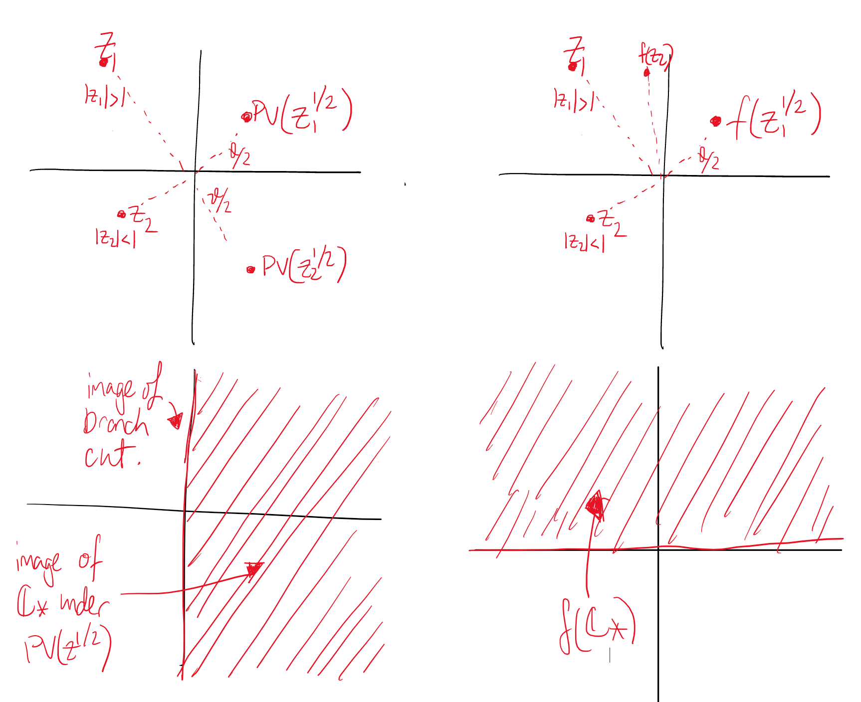Exercise: Repeat for (z-z_0)^{1/2}.

Trigonometric functions

B-C 37-39 (8Ed 34-35)

For x \in \mathbb R, \begin{aligned} e^{ix} &= \cos x + i\sin x \\ e^{-ix} &= \cos x - i \sin x\\ \implies \cos x &= \frac{e^{ix}+e^{-ix}}2\\ \implies \sin x &= \frac{e^{ix}-e^{-ix}}{2i} \end{aligned} We can use these expressions to define \cos and \sin on \mathbb C. Specifically, \cos z = \frac{e^{iz}+e^{-iz}}2\quad \text{and}\quad \sin z = \frac{e^{iz}-e^{-iz}}{2i}. This gives us the following properties: - \cos z = \cos (-z) - \sin z = - \sin (-z) - \cos(z+\xi) = \cos z \cos \xi - \sin z \sin \xi - \sin (z+\xi) = \sin z \cos \xi + \cos z \sin \xi - \sin^2 z + \cos^2 z = 1 (this does not imply that they are bounded in \mathbb C) - \sin (z+\pi/2) = \cos z - \sin (z-\pi/2) = -\cos z (these two proven using properties of exp)

Hyperbolic functions

On \mathbb R, the hyperbolic functions were \sinh x = \frac{e^x-e^{-x}}2\\ \cosh x = \frac{e^x + e^{-x}}2 Recall that \sinh is somewhat like a exaggerated cubic and \cosh is not unlike a steeper periodic parabola. Also, \cosh can be used to model a hanging cable with weight.

Similarly to the first trig functions, we can define the hyperbolic functions on \mathbb C as \cosh z = \frac{e^{z}+e^{-z}}2\quad \text{and}\quad \sinh z = \frac{e^{z}-e^{-z}}{2}. Interestingly, \sin (iy) = i \sinh y \quad \text{and}\quad \cos(iy) = \cosh y. Tke z = x and \xi = iy in the sum formulas and we get \begin{aligned} \sin(x+iy) &= \sin x \cos(iy) + \cos x + \sin (iy)\\ &= \sin x \cosh y + i \cos x \sinh y\\ \cos(x+iy) &= \cos x \cosh y - i\sin x \sinh y \end{aligned} Together, the two above equalities imply \sin(z+2\pi) = \sin z and \cos(z+2\pi) = \cos z. Additionally, we have \cosh^2 z = 1+\sinh^2 z and \begin{aligned} |\sin z|^2 &= \sin^2 x \cosh^2 y + \cos^2 x \sinh^2 y \\ &= \sin^2 x(1+\sinh^2y) +(1-\sin^2x)\sinh^2 y\\ &= \sin^2 x + \sinh^2 y\\ |\cos z|^2 &= \cos^2x + \sinh^2 y \end{aligned}

Recall that a function f : \Omega \to \mathbb Z is called bounded if there exists M such that |f(z)| \le M for all z \in \Omega. Note that there can exist unbounded functions with finite area.

Finally, \sin and \cos are unbounded on \mathbb C, because with a sufficiently large imaginary component they can become arbitrarily large.

Lecture 10 — Bounded Functions & Topology

Recall that we can have unbounded functions with bounded area.

Examples:

• f(z) = \xi is bounded.
• f(z) = 1/z is unbounded on \mathbb C_* and on \{z : 0 < |z| \le 1\} but bounded on \{z : |z| \ge 1\} and \{z : |z| = 1\}.
• f(z) = z is unbounded in \mathbb C but bounded on any bounded subset of \mathbb C.
• f(z) = \frac 1 {1+|z|} is bounded on \mathbb C.

Definition. A zero of a function is a value of z such that f(z) = 0.

For example, the zeros of \sin are n\pi + 0i for n \in \mathbb Z. This can be derived from the \sin(x+iy) = \sin x \cosh y + i \cos x \sinh y equation. Similarly, the zeros of \cos are (n+1/2)\pi. The zeros of \sinh and \cosh are n\pi i and (n+1/2)\pi i, respectively.

Inverse Trig Functions

If w = \arcsin z, then z = \sin w and \begin{aligned} z &= \sin w \\ &= \frac {e^{iw}-e^{-iw}}{2i} \frac{e^{iw}}{e^{iw}}\\ &= \frac{e^{2iw}-1}{2ie^{iw}}\\ \implies 2ie^{ze^{iw}} &= e^{2iw}-1\\ \implies (e^{iw})^2 - 2iz(e^{iw}) - 1& = 0 \end{aligned} We can solve this quadratic using the complex quadratic formula, which doesn’t use \pm but instead uses (\cdot)^{1/2} as a multi-valued square root. So, \begin{aligned} \implies e^{iw} &= \frac{2iz + (-4z^2 + 4)^{1/2}}{2} \\ &= iz + (1-z^2)^{1/2}\\ \implies iw &= \log(iz + (1-z^2)^{1/2})\\ w =\arcsin z&= -i\log(iz + (1-z^2)^{1/2}) \end{aligned} Note that we have a multi-valued logarithm and for each of those, a double-valued square root. This makes it a lot more fun than real numbers.

Example: \arcsin (-i) = -i\log(1+z^{1/2})=-i\log(1\pm\sqrt 2). So we need to consider two logarithms. \log(1+\sqrt 2) = \ln (1+ \sqrt 2) + 2n\pi i is relatively fine. Then, \begin{aligned} \log (1-\sqrt 2) &= \ln|1-\sqrt 2| + \arg(1-\sqrt 2)\\ &=\ln (\sqrt 2 - 1) + (2n+1)\pi i \end{aligned} Putting these together, we get \arcsin (-i) is -i(\ln(1+\sqrt 2)+2n\pi i) and -i(\ln(\sqrt 2-1)+(2m+1)\pi i) for n, m \in \mathbb Z.

Topology

Topology is the study of topos, space. Our basic building block is some ball around an arbitrary point in \mathbb C.

Definition. Given z_0 \in \mathbb C and \epsilon > 0, B_\epsilon(z_0) denotes the (open) ball of radius \epsilon about z_0, a.k.a. an \epsilon-neighbourhood of z_0. In set notation, B_\epsilon(z_0) = \{z : |z-z_0| < \epsilon\}. Similarly, \overline B_\epsilon(z_0) is the closed ball of radius \epsilon about z_0 (a closed \epsilon-neighbourhood of z_0) given by \{ z : |z-z_0| \le \epsilon\}. A deleted \epsilon-neighbourhood of z_0 is \{z : 0 < |z-z_0| < \epsilon\}.

Note that the only feature of \mathbb C used by this definition is |\cdot|, the modulus. That is, \begin{aligned} |z-z_0| &= \sqrt{(x-x_0)^2 + (y-y_0)^2} \\ &= \|(x,y)-(x_0,y_0)\|_{\mathbb R^2} \\ &= d((x,y), (x_0,y_0))_\mathbb R \\ &= d(z, z_0)_\mathbb C \end{aligned} This has obvious analogues to \mathbb R with d(x,y)_\mathbb R = |x-y| being the absolute value distance. Balls in \mathbb R are just intervals.

Definition. Given \Omega \subseteq \mathbb C, z \in \mathbb C is an interior point of \Omega if there exists \epsilon > 0 such that B_\epsilon(z) \subset \Omega. Note that this implies B_{\epsilon'}(z) \subset \Omega for all 0<\epsilon' < \epsilon.

Definition. z \in \mathbb C is an exterior point of \Omega if there exists \epsilon > 0 such that B_\epsilon(z) \cap \Omega = \emptyset.

Definition. z \in \mathbb C is a boundary point of \Omega if for all \epsilon > 0, B_\epsilon(z) \cap \Omega \ne \emptyset and B_\epsilon(z) \cap \Omega^c \ne \emptyset. That is, any \epsilon-neighbourhood around z contains points inside and outside \Omega. Here, $^c $ denotes the complement, that is \mathbb C \setminus \Omega.

Lecture 11 — Topology Definitions

Definition. The boundary of \Omega, denoted \partial \Omega, is defined as \{z \in \mathbb C : z \text{ is a boundary point}\}.

Recall that interior points are in \Omega and exterior points are in \Omega^c. What about the boundary points?

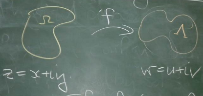
Let’s look at a circle \Omega = \{z : |z| = 1\}. In this case, we have \partial \Omega = \Omega. Let’s consider a blob:

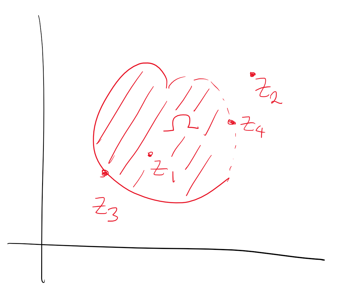
Here, z_1 is an interior point, z_2 is an exterior point, z_3 is a boundary point in \Omega, and z_4 is a boundary point not in \Omega.

Definition. \operatorname{Int}\Omega is the interior of \Omega, the set of all interior points. \operatorname{Ext}\Omega is the exterior of \Omega, the set of all exterior points.

Definition. \Omega is open if \Omega = \operatorname{Int}\Omega, and \Omega is closed if \partial \Omega \subseteq \Omega.

Examples:

• Consider the open unit ball, \Omega_1 = B_1(0) = \{z : |z| < 1\}. For this set, \operatorname{Int} \Omega_1 = \Omega_1, \operatorname{Ext}\Omega_1 = \{z : |z| > 1\}, \partial \Omega_1 = \{z : |z| = 1\}. Note that this means \Omega_1 is open.

• Consider the closed unit ball, \Omega_2 = \overline{B}_1(0). Here, \operatorname{Int}\Omega_2 = \Omega_1, \operatorname{Ext}\Omega_2 = \operatorname{Ext}\Omega_1, and \partial \Omega_2 = \partial \Omega_1. This means \Omega_2 is closed.

• Consider \Omega_3 = \{z : 0 < |z| \le 1\}. \operatorname{Int} \Omega_3 = \{ z : 0 < |z| < 1\}, \operatorname{Ext} \Omega_3 = \operatorname{Ext} \Omega_1, \partial \Omega_3 = S^1 \cup \{0\}. This is neither open nor closed.

Note that \Omega_1 is open and \Omega_1^c is closed. \Omega_2 is closed and \Omega_2^c is open. Both \Omega_3 and \Omega_3^c are neither open nor closed.

Definition. A set which is both closed and open is called clopen.

Definition. A set \Omega \subseteq \mathbb C is called connected if there do not exist non-empty, open, disjoint sets \Omega' and \Omega'' such that \Omega \subseteq \Omega' \cup \Omega'' and \Omega' \cap \Omega \ne \emptyset and \Omega'' \cap \Omega \ne \emptyset.

That is, we can’t find two ‘separated’ sets which together contain all of \Omega and each contain parts of \Omega.

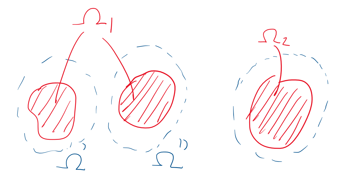
Above, \Omega_1 is disconnected because we can find such \Omega' and \Omega''. However, \Omega_2 is connected.

Lecture 12 — Path Connected, Domains and Limits

Definition. A set \Omega \subseteq \mathbb C is piecewise affinely path connected if any two points in \Omega can be connected by a finite number of line segments in \Omega, joined end to end.

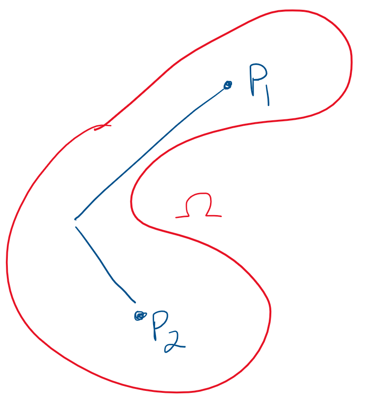
For open sets in \mathbb C, this is equivalent to the original definition of connected. (This will not be proved in MATH3401.)

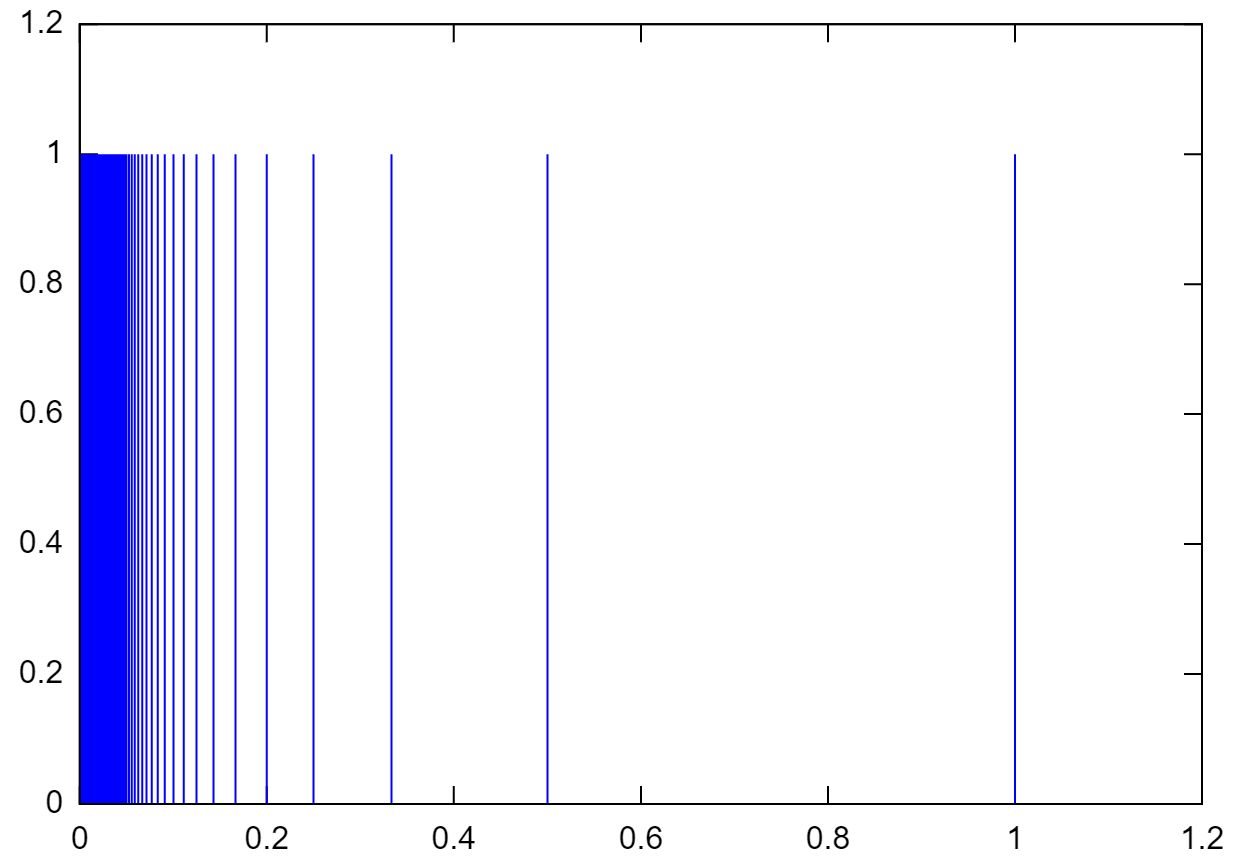
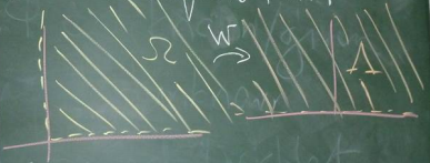
However, it is not so in general. For example, there is a comb space which is connected but not path connected. This is connected because we cannot find open sets

Claim. If \Omega_1 and \Omega_2 are open subsets of \mathbb C, then so is \Omega_1 \cap \Omega_2.

Proof. If \Omega_1 \cap \Omega_2 =\emptyset, then we are done because the empty set is open. Otherwise, for any z \in \Omega_1 \cap \Omega_2, there exist \epsilon_1, \epsilon_2 > 0 such that B_{\epsilon_1}(z) \subseteq \Omega_1 and B_{\epsilon_2}(z) \subseteq \Omega_2. Take \epsilon = \min \{\epsilon_1, \epsilon_2\}. Then, B_\epsilon(z) \subseteq \Omega_1 and B_\epsilon(z) \subseteq \Omega_2 which implies B_\epsilon(z) \subseteq \Omega_1 \cap \Omega_2. Since z was arbitrary and this is the definition of interior point, we see that \operatorname{Int}(\Omega_1 \cap \Omega_2) = \Omega_1 \cap \Omega_2. Therefore, \Omega_1 \cap \Omega_2 is open. \square

Definition. A domain is an open, connected subset of \mathbb C. A region is a set whose interior is a domain.

Definition. A point z \in \mathbb C is called an accumulation point of \Omega \subseteq \mathbb C if any deleted neighbourhood of z intersects \Omega. Note that z need not be in \Omega.

Examples:

• If \Omega = \{i/2^n\}_{n \in \mathbb N}, then the only accumulation point is 0.
• If \Omega = B_1, then the set of accumulation points is \overline B_1.

Limits

B-C 15-16.

Definition. Let f be a complex-valued function defined on a deleted neighbourhood of z_0 \in \mathbb C. Then, we say \lim_{z \to z_0} f(z) = w_0 if for all \epsilon > 0, there exists \delta > 0 such that 0 < |z-z_0| < \delta \implies |f(z) - w_0| < \epsilon. Note that f does not need to be defined at z_0.

Examples:

• If f(z) = \begin{cases} 0 & z\ne 0 \\ 1337 & z = 0\end{cases}, then \lim_{z \to 0} f(z) = 0.
• \lim_{z \to 0} \sin z / z = 1.

Remark. If a limit exists, then it is unique.

Limit Theorems

B-C 17 (8 Ed 16)

Suppose z=x+iy and f(z) = u(x,y)+iv(x,y). Let z_0 = x_0 + iy_0 and w_0 = u_0 + iv_0.

Theorem 1. \lim_{z\to z_0} f(z)= w_0 \iff \begin{cases} \lim_{(x,y)\to(x_0, y_0)} u(x,y) = u_0, & \text{and}\\ \lim_{(x,y)\to(x_0, y_0)} v(x,y) = v_0. \end{cases} Theorem 2. (Non-exciting facts about operations of limits.) Suppose \lim_{z \to z_0}f(z) = w_0, \lim_{z \to z_0}g(z) = \xi_0 and \lambda \in \mathbb C. Then, \begin{align} \lim_{z \to z_0}(f \pm g)(z) &= w_0 \pm \xi_0 \tag{1}\\ \lim_{z \to z_0}(\lambda f)(z) &= \lambda w_0 \tag{2}\\ \lim_{z \to z_0}(fg)(z) &= w_0\xi_0 \tag{3}\\ \lim_{z \to z_0}\frac{f(z)}{g(z)} &=\frac{ w_0}{\xi_0}\qquad\text{ if } \xi_0 \ne 0\tag{4} \end{align} Not that \lim_{z\to z_0}g(z) = \xi_0 and \xi_0 \ne 0 implies g(z) \ne 0 within a neighbourhood of z_0.

Lecture 13 — Limits, Continuity and Differentiability

Recall the comb space, space with vertical lines of length 1 at x = 1/2^i and a horizontal line of length 1, with the origin removed. This is not path affinely finite path connected because we cannot move through the origin.

However, it is connected because any open set containing the x=0 line must extend some distance towards the other lines, hence containing the rest of the comb lines. So there do not exist two disjoint open sets which contain this comb, and it’s connected.

Limits at infinity

Recall in \mathbb R that \lim_{x\to x_0}f(x) = \infty means: given M> 0, \exists \delta > 0 such that 0 < |x-x_0| < \delta implies f(x) > M.

In \mathbb C, a neighbourhood of z_0 \in \mathbb C is a ball and a neighbourhood of \infty has the form \{z : |z| > M\}. Note that in the Riemann sphere model, this would be some region around the “north pole”.

So, “close to \infty” \iff |z| is large \iff 1/|z| is small. Keeping that in mind, this means \begin{aligned} \lim_{z \to z_0} f(z) = \infty &\iff \lim_{z \to z_0} \frac 1 {f(z)} = 0\\ \lim_{z \to \infty} f(z) = w_0 &\iff \lim_{z \to 0} f(1/z) = w_0 \\ \lim_{z \to \infty} f(z) = \infty &\iff \lim_{z \to 0} \frac 1{f(1/z)} = 0 \end{aligned} Examples:

• Show \lim_{z \to -1} \frac{iz+3}{z+1} = \infty. We need to show \lim_{z \to -1} \frac{z+1}{iz+3} = 0 which is true because the function is continuous at -1.
• Compute \lim_{z \to \infty} \frac{2z^3-1}{z^2-1}. This might be \infty so we need to show \lim_{z \to 0} \frac{z^{-2}-1}{2z^{-3}-1} = \lim_{z \to 0}\frac{z-z^3}{2-z^3} =0. The limit exists and is \frac 0 2 = 0.

Continuity & Differentiability

B.C. 19 (8 Ed 18)

Let f be defined in some neighbourhood of z_0.

Definition. We say f is continuous at z_0 if \lim_{z \to z_0} f(z) = f(z_0). That is, given \epsilon > 0 there exists \delta > 0 such that |z-z_0| < \delta \implies |f(z) - f(z_0)| < \epsilon.

Basic results

• If f : \Omega \to U and G : U \to W are both continuous, then so is g \circ f : \Omega \to W, where (g \circ f)(z) = g(f(z)).
• If f is continuous and non-zero at z_0, then there exists B_\epsilon(z_0) such that f(z) \ne 0 on this ball.
• f : x + iy \mapsto u(x,y) + iv(x,y) is continuous if and only if u and v are continuous. That is, it must be continuous in the component functions.

Differentiability

Recall that f : \Omega \subseteq \mathbb R \to \mathbb R is differentiable if \lim_{h \to 0} \frac{f(x+h)-f(x)}h exists, and the limit defines f'(x) in \mathbb R.

Definition. For f : \Omega \subseteq \mathbb C\to \mathbb C is differentiable if \lim_{\xi \to 0} \frac{f(z_0+\xi)-f(z_0)}\xi exists and the limit defines f'(z_0).

This definition implies f'(z_0) = \lim_{\Delta z \to 0} \frac{f(z_0+\Delta z) - f(z_0)}{\Delta z}. Writing w = f(z) and \Delta w = f(z_0 + \Delta x) - f(z_0), we can write f'(z_0) = \lim_{\Delta z \to 0} \frac{\Delta w}{\Delta z} = \frac {dw}{dz}(z_0). These are equivalent ways to write the derivative.

Lecture 14 — Derivatives and Complex Differentiation

Example: Take the derivative of f(z) = 4z^2 from first principles. Put w = f(z) and take z_0 \in \mathbb C. \begin{aligned} \lim_{\Delta z \to 0} \frac{\Delta w}{\Delta z} &= \lim_{\Delta z \to 0} \frac{f(z_0 + \Delta z) - f(z_0)}{\Delta z} \\ &= \lim_{\Delta z \to 0} \frac{4(z_0 + \Delta z)^2 - 4z_0^2}{\Delta z} \\ &= \lim_{\Delta z \to 0} \frac{4z_0^2 + 8z_0\Delta z + 4(\Delta z)^2 - 4z_0^2}{\Delta z}\\ &= 8z_0\\ \implies f'(z) &= 8z \end{aligned}

Example: For f(z) = |z|^2, f' doesn’t exist except at z=0. This is a very different situation from the case in \mathbb R, where the function is differentiable everywhere.

B.C. 23 Ex 2 (8 Ed 22 Ex 2)

Note. Differentiability implies continuity, but the converse does not hold. An example of the converse failing is |z|^2 or |z|.

Formulae (compare to f : \mathbb R \to \mathbb R)

\begin{aligned} \frac{d}{dz}(c) &= 0\qquad c \in \mathbb C \\ \frac{d}{dz}\,z^n &= n z^{n-1} \quad n \in \mathbb Z\\ \frac{d}{dz} \,e^z &= e^z \\ \frac{d}{dz} \,\sin z &= \cos z \\ \frac{d}{dz} \,\cos z &= -\sin z \end{aligned}

The usual rules apply. For f, g differentiable, \begin{aligned} (f \pm g)' &= f' \pm g' \\ (fg)' &= fg' + f'g \\ (f/g)' &= \frac{gf' - fg'}{f^2} \quad g \ne 0 \end{aligned} We also have the chain rule: if f is differentiable at z_0 and g is differentiable at f(z_0), then the composition g \circ f is differentiable at z_0 and the derivative is (g\circ f)'(z_0) = g'(f(z_0))f'(z_0) and this can be written as \frac{dg}{dz} = \frac{dg}{dw} \frac{dw}{dz}\quad \text{where } w = f(z).

Cauchy-Riemann

Let z = x+iy and suppose f : z \mapsto w = u(x,y) + iv(x,y) is differentiable at z_0 = x_0 + iy_0. Set \Delta z = \Delta x + i \Delta y, then f'(z_0) = \lim_{\Delta z\to 0} \frac{\Delta w}{\Delta z}.

Key point: If the derivative exists, its value is independent of how \Delta z \to 0.

Note that \begin{aligned} \Delta w = f(z_0 + \Delta z) - f(z_0) &= u(x_0 + \Delta x, y_0 + \Delta y) + iv (x_0 + \Delta x, y_0 + \Delta y) - u(x_0,y_0) - iv(x_0, y_0) \end{aligned} We can decompose the limit into real and imaginary, \begin{aligned} f'(z_0) &= \lim_{(\Delta x, \Delta y) \to (0,0)} \operatorname{Re}\left(\frac{\Delta w} {\Delta z}\right) + i \lim_{(\Delta x, \Delta y) \to (0,0)}\operatorname{Im}\left(\frac{\Delta w} {\Delta z}\right). \end{aligned} These limits must still be independent of the path (\Delta x, \Delta y) \to (0,0). To start, let (\Delta x, \Delta y) \to (0,0) along the x-axis, i.e. along (\Delta x, 0) for \Delta x \ne 0. So, \begin{aligned} \frac{\Delta w}{\Delta z} &= \frac{u(x_0 + \Delta x, y_0) - u(x_0, y_0)}{\Delta x} + i\frac{v(x_0 + \Delta x_0, y_0) - v(x_0, y_0)}{\Delta x} \end{aligned} which implies (below, u_x is the partial derivative of u w.r.t. x) \begin{aligned} \lim_{(\Delta x, \Delta y) \to (0,0)} \operatorname{Re}\left(\frac{\Delta w} {\Delta z}\right) &= u_x(x_0, y_0) = \frac{\partial u}{\partial x}(x_0, y_0) \\ \lim_{(\Delta x, \Delta y) \to (0,0)} \operatorname{Im}\left(\frac{\Delta w} {\Delta z}\right) &= v_x(x_0, y_0) = \frac{\partial v}{\partial x}(x_0, y_0) \end{aligned} We can derive similar expressions for \Delta z \to 0 along the y-axis. For this, we get \begin{aligned} \frac{\Delta w}{\Delta z} &= \frac{u(x_0, y_0 + \Delta y) - u(x_0, y_0)}{i\Delta y} + i\frac{v(x_0, y_0+ \Delta y) - v(x_0, y_0)}{i\Delta y} \end{aligned} Being careful with the i, we get \begin{aligned} \lim_{(\Delta x, \Delta y) \to (0,0)} \operatorname{Re}\left(\frac{\Delta w}{\Delta z}\right) &= v_y(x_0, y_0) \\ \lim_{(\Delta x, \Delta y) \to (0,0)} \operatorname{Re}\left(\frac{\Delta w}{\Delta z}\right) &= -u_y(x_0, y_0) \\ \end{aligned} Together, because the \Delta z \to 0 must be path independent and we’ve found the value along two paths, these must coincide. This gives is the Cauchy-Riemann equations.

Theorem. (Cauchy-Riemann equations) If f = u+iv is differentiable at z_0 = x_0 + iy_0, then u_x = v_y and -v_x= u_y at (x_0, y_0).

Note. We have shown that C/R are necessary for complex differentiability, but they are not sufficient. There are sufficient conditions.

Sufficient conditions

If we know

• f is defined in a neighbourhood of z_0,
• u_x, u_y, v_x, v_y are defined and continuous in a neighbourhood of (x_0, y_0), and
• C/R hold at (x_0, y_0),

then f'(z_0) exists.

Note that there are no is in this board; it is a statement on functions of \mathbb R^2.

Remark. There are no necessary and sufficient conditions for complex differentiability. Otherwise, we would have reduced complex analysis to \mathbb R^2 analysis (how boring!).

Lecture 15 — Wirtinger Operators and Analytic Functions

What does Cauchy-Riemann mean in polar coordinates? Take z = x+iy = re^{i\theta} so x = r \cos \theta and y = r \sin \theta. By the chain rule, we get \begin{aligned} u_r &= u_x \cos \theta + u_y \sin \theta \\ u_\theta &= -u_x r \sin \theta + u_y r \cos \theta \\ v_r &= v_x \cos \theta + v_y \sin \theta \\ v_\theta &= v_x r \sin \theta + v_y r \cos \theta \end{aligned} We can derive C/R in polar coordinates as r u_r = v_\theta and u_\theta = -r v_r.

Therefore, if f' exists, then f' = u_x + iv_x. By using the polar coordinates expression, we also get f'(z) = e^{-i\theta}(u_r + iv_r).

Wirtinger operators

Formally, we are going to change variables from (x,y) to (z, \bar z), where z = x+iy and \bar z = x-iy. This means that x = (z + \bar z)/2 and y = (z - \bar z)/(2i).

This derivation makes use of the multivariate chain rule. Specifically, if x(t) and y(t) are differentiable functions of t and z = f(x,y) is a differentiable function of x and ythen z = f(x(t),y(t)) is differentiable and \frac{dz}{dt} = \frac{\partial z}{\partial x}\frac{\partial x}{\partial t} + \frac{\partial z}{\partial y}\frac{\partial y}{\partial t}.

\begin{aligned} \frac{\partial f}{\partial x} &= \frac{\partial f}{\partial z}\frac{\partial z}{\partial x} + \frac{\partial f}{\partial \bar z} \frac{\partial \bar z}{\partial x} \\ &= \frac {\partial f}{\partial z} + \frac {\partial f}{\partial \bar z} \\ \frac{\partial f}{\partial y} &= \frac{\partial f}{\partial z}\frac{\partial z}{\partial y} + \frac{\partial f}{\partial \bar z} \frac{\partial \bar z}{\partial y} \\ &= i\frac {\partial f}{\partial z} -i \frac {\partial f}{\partial \bar z} \\ \end{aligned}

Then, \begin{aligned} \frac{\partial f}{\partial x} - i\frac{\partial f}{\partial y} &= 2 \frac{\partial f}{\partial z} \implies \frac{\partial }{\partial z} = \frac 1 2 \left(\frac \partial {\partial x} - i \frac \partial {\partial y}\right) \\ \frac{\partial f}{\partial x} + i\frac{\partial f}{\partial y} &= 2 \frac{\partial f}{\partial \bar z} \implies \frac{\partial }{\partial \bar z} = \frac 1 2 \left(\frac \partial {\partial x}+ i \frac \partial {\partial y}\right) \end{aligned} \frac{\partial}{\partial z} and \frac{\partial}{\partial \bar z} are called the Wirtinger operators.

Example: Consider f(z) = z^n = (x+iy)^n. Then, \begin{aligned} \frac{\partial f}{\partial z} &= \frac 1 2 \left(\frac \partial {\partial x} - i \frac \partial {\partial y}\right)(x+iy)^n \\ &= \frac 1 2(n(x+iy)^{n-1} -i^2n(x+iy)^{n-1}) \\ &= \frac 1 2(n(x+iy)^{n-1} +n(x+iy)^{n-1})\\ &= n(x+iy)^{n-1} = nz^{n-1}=f'(z) \\ \frac{\partial f}{\partial \bar z} &= 0\quad \text{(follows from above)} \end{aligned}

For f = u+iv complex differentiable, \begin{aligned} \frac 1 2 \frac{\partial f}{\partial x} &= \frac 1 2 (u_x + iv_x) \overset{\text{CR}}= \frac 1 2 (v_y -iu_y) \\ &= -\frac i 2 (u_y + iv_y) = -\frac i 2\frac{\partial f}{\partial y} \end{aligned} So C/R holds if and only if \frac{\partial f}{\partial \bar z} = 0. This is version II of the Cauchy-Riemann equations.

But why is this partial derivative equal to the full derivative? From f' = u_x + iv_x, \begin{aligned} \frac{df}{dz} &= u_x + iv_x = \frac{\partial f}{\partial x} \\ &= -i \frac{\partial f}{\partial y}\quad \text{(by CR)} \\ &= \frac 1 2 \left(\frac{\partial f}{\partial x} -i \frac{\partial f}{\partial y}\right) \\ &= \frac{\partial f}{\partial z} \end{aligned} Example 1: Find f'(z) for f(z) = e^z. First, we check the sufficient conditions for f' to exist. Writing f(z) = u+iv = e^{x+iy} = e^x(\cos y + i \sin y), it is defined on \mathbb C. Moreover, the components are u = e^x \cos y and v = e^x \sin y which have partials defined and continuous on \mathbb C. Then, we need to check C/R by testing u_x = v_y and u_y = -v_x or just checking \frac{\partial f}{\partial \bar z} = 0.

Example 2: When is g(z) = |z|^2 differentiable? Note that g(z) = z \bar z = x^2 + y^2. Checking C/R II, \frac{\partial g}{\partial \bar z} = 0 \implies z = 0, so g cannot be differentiable for z \ne 0 because C/R is necessary. At z = 0, we check the sufficient conditions. It is easy to show that u, v, u_x, v_x, u_y, v_y are defined and continuous on a neighbourhood of 0. Therefore, g'(0) = 0.

Exercise: Go through the same exercise for z \mapsto 1/z on \mathbb C_*.

Definition. A function f : \Omega \to \mathbb C is analytic at z_0 if f is differentiable on a neighbourhood of z_0.

Definition. A function is singular at z_0 if it is not analytic at z_0 but is analytic at some point in any neighbourhood of z_0. For example, f(z) = 1/z is analytic on \mathbb C_* and singular at 0.

That is, given B_\epsilon(0), f is analytic on B_{\epsilon'}(z_0) for some z_0 \in B_\epsilon(0) and \epsilon' < |z_0|.

Definition. A function is entire if it is analytic on all of \mathbb C. For example, polynomials, sine, cosine, exponential, etc.

Note: If a function is differentiable at precisely one point, it is not analytic there or anywhere (e.g. |z|^2).

Also, note that we are calling once-differentiable functions analytic. In real analysis, analytic functions were smooth and equal to their power series (infinitely differentiable). What’s going on?

Lecture 16 — Examples of Derivatives and Taylor Series

Mid-semester exam: Wednesday 22/04/2020 9am.

Remember from real analysis that we have functions differentiable once but not twice.

Continuing with derivatives, consider \frac{d}{dz} \log z where |z| > 0. Recall that in \mathbb C, \log z = \ln |z| + i \arg z=\ln r + i\theta. Looking at the second expression in its components, u = \ln r and v = \theta so u_r = 1/r, u_\theta = 0, v_r = 0 and v_\theta = 1. Checking C/R in polar coordinates, we need ru_r = v_\theta \quad \text{and}\quad u_\theta = -rv_r which we do have. We need to make \log a function so it can be continuous; we need to choose a branch. Pick a subset of \mathbb C_* such that \alpha < \theta < \alpha + 2\pi then \log is differentiable. From Lecture 15, \frac d{dz} \log z = e^{-i\theta}(u_r + iv_r) = e^{-i\theta}/r = 1/z. For example, \frac d{dz} \operatorname{Log} z = 1/z for -\pi < \operatorname{Arg}z < \pi and |z| > 0.

For f(z) = z^c where c \in \mathbb C_* is fixed, we have f(z) = \exp (c \log z) and f'(z) = c\exp (c \log z)/z by the chain rule and using the derivative of \log. We can also write this as z^c c/z = cz^{c-1} which is valid on any domain of the form \{z : |z| > 0, \alpha < \arg z < \alpha + 2\pi\}, due to the branch cut of \log.

Remark: Try this for g(z) = c^z.

Notation from real analysis

Given \Omega \subseteq \mathbb R^n,

• C(\Omega) = C^0(\Omega) is the set of continuous functions \Omega \to \mathbb R.
• C^k(\Omega) is the set of functions whose derivatives/partial derivatives of order 0, 1, \ldots, k exist and are continuous. (0-th order derivative is f itself.)
• C^\infty(\Omega) is the set of functions whose derivatives/partial derivatives exist and are continuous. That is, smooth functions.
• C^\omega(\Omega) is the set of real analytic functions. That is, for all x_0 \in \Omega,
  • 1. f has a power series expansion about x_0 (namely, its Taylor series), and
  • 2. f is given by its power series expansion (i.e. the power series converges to f on some neighbourhood of x_0.)

Note that (i) implies f is smooth, and in \mathbb R^n, (i) does not imply (ii).

Example: Consider an example to illustrate this past point. f(x) = \begin{cases} e^{-1/x^2} & x >0 \\ 0 & x \le 0 \end{cases} Then, f^{(n)}(x) exists for all x \ne 0 trivially and f^{(n)}(0) = 0 for all n. Also, f^{(n)} is continuous on \mathbb R. However, the Taylor series of f about 0 is \sum_{n=0}^\infty \frac{f^{(n)}(0) x^n}{n!} \equiv 0 so f is not equal to its Taylor series in a neighbourhood of 0. Therefore, f \in C^\infty(\mathbb R) but f \notin C^\omega(\mathbb R).

In real analysis, we have C^\omega \subsetneq C^\infty \subsetneq \cdots \subsetneq C^{1000} \subsetneq \cdots \subsetneq C^1 \subsetneq C^0. Next, we will be moving onto integration but there are some problems. There was the intuition of ‘area’ but how does this translate to \mathbb C? We could look at something like a two-dimensional volume under a hypersurface but that doesn’t really work. Instead, we can revert to a complex valued function of real parameters. Next lecture, we will see why this makes sense and how it leads to the familiar integration.

Lecture 17 — Integration, Rules, FToC, Contours

We want integration to give us some notion of (signed) as well as reversing differentiation, with the goal of building up the fundamental theorem of calculus.

Integration

B-C §41-43 (8 Ed §37-39)

Consider a \mathbb C-valued function of one real variable. That is, w(t) = u(t) + iv(t) for t \in \mathbb R. Define w'(t) = u'(t) + iv'(t).

The usual rules for real-valued differentiation apply:

• (cw)' = cw'
• (w_1 \pm w_2)' = w_1' \pm w_2'
• \frac d {dt} e^{ct} = ce^{ct}
• product rule
• quotient rule
• etc.

We can also define definite and indefinite integrals for such functions. For a, b \in \mathbb R, \begin{aligned} \int_a^b w(t)\, dt &= \int_a^b u(t)\,dt + i\int_a^bv(t)\,dt \\ \operatorname{Re}\left(\int_a^b w(t)\,dt\right) &= \int_a^b \operatorname{Re}(w(t))\,dt \\ \operatorname{Im}\left(\int_a^b w(t)\,dt\right) &= \int_a^b \operatorname{Im}(w(t))\,dt \end{aligned} \int_0^\infty w(t)\,dt and similar can be defined analogously. The above expressions certainly make sense if w is continuous, that is w \in C^0([a,b]).

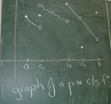
Somewhat more generally, it also holds for piecewise continuous functions on [a,b]. That is, w such that there exist c_1 < c_2 < \cdots < c_n \in (a,b) such that

• 1. w is continuous on each of (a, c_1), (c_1, c_2), \ldots, (c_n, b),
• 2. \lim_{t \to c_j^-} w(t) and \lim_{t\to c_j^+}w(t) both exist (but they need not coincide), and
• 3. \lim_{t \to a+}w(t) and \lim_{t \to b^-} w(t) both exist.

Of course, the limits existing for w imply the limits exist for u and v.

Suppose there exists W(t) = U(t) + iV(t) such that W' = w on [a,b]. Then, the fundamental theorem of calculus holds, in the form of \int_a^b w(t)\,dt = W(b) - W(b). The next estimate is crucial.

Lemma. Suppose w = u+iv is piecewise continuous on [a,b]. Then, \left|\int_a^b w(t)\,dt\right|\le \int_a^b \left|w(t)\right|\,dt. Proof. If \int_a^b w(t)\,dt = 0, then the left is 0 and right is \ge 0 so we are done. Otherwise, there exists r > 0 and \theta_0 \in \mathbb R such that \int_a^b w(t)\,dt = re^{i\theta_0} which implies \left|\int_a^b w(t)\,dt\right| = r. Then, \begin{aligned} \int_a^b w(t)\,dt &= re^{i\theta_0}\\ \int_a^b e^{-i\theta_0} w(t)\,dt &= r\\ \implies r=\int_a^b e^{-i\theta_0} w(t)\,dt &=\operatorname{Re}\left(\int_a^b e^{-i\theta_0} w(t)\,dt\right) \\ &= \int_a^b \operatorname{Re}\left(e^{-i\theta_0}w(t)\right)\,dt \end{aligned} However, \operatorname{Re}\left(e^{-i\theta_0}w(t)\right) \le \left|e^{-i\theta_0}w(t)\right| = |w(t)| because \left|e^{-i\theta_0} \right|= 1. Combining this with the expression for \left|\int_a^b w(t)\,dt\right| = r from earlier, \left|\int_a^b w(t)\,dt\right| = r \le \int_a^b \operatorname{Re}\left(e^{-i\theta_0}w(t)\right)\,dt \le \int_a^b \left|w(t)\right|\,dt. \square

Contours and arcs

A contour is a parametrised curve in \mathbb C. Given x(t), y(t) continuous on [a,b] \to \mathbb R, z(t) = x(t) + iy(t), \quad a \le t \le b defines an arc in \mathbb C.

This is both a set of points z([z,b]), called the trace of the arc, and also a recipe for drawing the arc (the parametrisation).

Lecture 18 - Jordan Curves, Simple Closed Contours

Recall that z(t) = x(t) + iy(t) for t \in [a,b]. The parameter t can be thought of as time.

Definition. A Jordan arc (or simple arc) does not intersect itself. That is, z(t_1) \ne z(t_2) for t_1 \ne t_2.

Definition. A Jordan curve (or simple closed curve) is a Jordan arc that has the property z(a) = z(b).

Example 1: z = \begin{cases}t + it & 0 \le t \le 1 \\ t + i & 1 < t \le 2\end{cases} is a simple arc, whose trace is the graph of the points. The arc would be traced out with a ‘speed’ of \sqrt2 between 0 and 1 because it covers a distance of \sqrt2 in 1 time unit.

Example 2: z = z_0 + Re^{i\theta} for 0 \le \theta \le 2\pi is an arc whose trace is a circle, centred at z_0 of radius R.

Example 3: z = z_0 + Re^{-i\theta} for 0 \le \theta \le 2\pi traces the same circle, but in the opposite direction. We use a negative in the exponent to allow the parameter to be increasing (fitting the time analogy).

Example 4: z = z_0 + Re^{2i\theta} for 0 \le \theta \le 2\pi again has the same trace, but it “covers” the circle twice.

In these examples, 2 and 3 are Jordan curves and 4 is not.

Definition. An arc/curve is called differentiable if z'(t) exists (at all t \in (a,b) for an arc, and at t \in [a,b] for a curve).

Definition. If z' exists and is continuous, then \int_a^b |z'(t)|\,dt exists and defines the arc length.

This is crucial because the length of an arc does not depend on the particular parametrisation. More specifically, if z(t) is any parametrisation of the image arc, we can define another one by t = \Phi(\tau) with \Phi(\alpha) = a and \Phi(\beta) = b such that \Phi \in C([\alpha, \beta]) and \Phi' \in C((\alpha, \beta)). Then, z(t) = Z(\tau) = z(\Phi(t)).

We will prove that the arc length is the same. Assume \Phi(\tau) > 0 for all \tau (that is, we always move forwards in time). Then, \begin{aligned} \int_a^b|z'(t)|\,dt &= \int_\alpha^\beta |z'(\Phi(\tau))| \Phi'(\tau)\,d\tau \\ &= \int_\alpha^\beta \left|Z'(\tau)\right|\,d\tau \end{aligned} which implies arc length is independent of parametrisation.

Definition. A contour is an arc/curve/Jordan curve such that z is continuous and z is piecewise differentiable. Additionally, if initial and final values coincide and there are no other self-intersections, it is a simple closed contour.

Theorem (Jordan curve theorem). Any simple closed contour divides \mathbb C into three parts:

• 1. on the curve,
• 2. inside the curve, and
• 3. outside the curve.

Although it seems obvious, this is actually more complex. Consider a Möbius strip. This would take about 8 lectures to prove, so we’ll trust Jordan on this one.

Remark: The theorem still holds if we remove the requirement that z is piecewise differentiable. This leads to very freaky things such as space-filling curves.

Contour integrals

Given a contour C, a contour integral is written \begin{aligned} \int_C f(z)\,dz \quad \text{ or }\quad \int_{z_1}^{z_2} f(z)\,dz. \end{aligned} We can write the second expression if we know:

• 1. the integral is independent of the path z_1 to z_2 (e.g. integrating a conservative field), or
• 2. path is understood.

Suppose the contour C is specified by z(t) with z_1 = z(a) and z_2 = z(b), with a \le t \le b, and suppose f is piecewise continuous on C. Then (reminiscent of line integrals), \int_C f(z)\,dz = \int_a^b f(z(t))z'(t)\,dt.

Glossary

• arc — z(t) = x(t) + iy(t) for a \le t \le b with x and y continuous on this interval.
• simple — no self intersections.
• closed curve — a curve which starts and ends at the same points.
• smooth — a differentiable arc with z' continuous on [a,b] and non-zero on (a,b).
• contour — an arc/curve/simple closed curve with z continuous and piecewise differentiable, alternatively a finite number of smooth arcs joined end to end.

Lecture 19 — Contour Integrals

Recall that an arc is made up of the trace, the image of points, and the parametrisation, a way of driving along the curve.

Suppose C is a contour given by z(t) for t \in [a,b] with z_1 = z(a) and z_2 = z(b). Suppose f is piecewise continuous on C.

Contour integrals

Basic properties

• The contour integral is linear: \begin{aligned} \int_C (\alpha f)(z)\,dz &= \alpha \int_C f(z)\,dz \quad\text{ for }\alpha \in \mathbb C\\ \int_C(f+g)(z)\,dz &= \int_C f(z)\,dz + \int_Cg(z)\,dz \end{aligned}

• C_1 + C_2 defines a contour only when the end of C_1 coincides with the start of C_2.

• -C is defined as w(t) = z(-t) for -b \le t \le -a. Using the change of parameter formula, we can show that \int_{-C}f(z)\,dz = -\int_C f(z)\,dz. Hence, C_1 - C_2 = C_1 + (-C_2). This means the end of C_1 has to be the start of -C_2 (i.e. the end of C_2).

Example: Evaluate I = \int_C \bar z\,dz where C is given by z(\theta) = 2e^{i\theta} for -\pi/2 \le \theta \le \pi/2. This traces the right half of a circle with radius 2 counter-clockwise. We check that C is continuous on C (indeed, differentiable) and f is continuous on C. Note that z'(\theta) = 2ie^{i\theta}. Then, \begin{aligned} \implies I &= \int_{-\pi/2}^{\pi/2} f(z(\theta)) z'(\theta)\,d\theta \\ &= \int_{-\pi/2}^{\pi/2}\overline{(2e^{i\theta})}2ie^{i\theta}\,d\theta \\ &= 4i\int_{-\pi/2}^{\pi/2}{e^{-i\theta}}e^{i\theta}\,d\theta \\ &= 4i\int_{-\pi/2}^{\pi/2}\,d\theta \\ &= 4\pi i \end{aligned} On C, z \bar z = 4 which implies \bar z = 4/z. As a corollary, \int_C \frac{dz}z = \pi i. See §45 (8 Ed §41) for more examples.

Antidifferentiation

Let D be a domain in \mathbb C (that is, an open connected subset of \mathbb C).

Definition. An antiderivative of f on D is F such that F'(z) = f(z) on D.

Theorem. The following three are equivalent:

• 1. f has an antiderivative on D,
• 2. for any z_1, z_2 \in D and any contour C from z_1 to z_2 in D, the integral \int_C f(z)\,dz is independent of C, and
• 3. for any closed contour C in D, it holds that \int_C f(z)\,dz = 0.

Proof. (i) to (ii) follows from the fundamental theorem of calculus. For (ii) to (iii), take a closed contour C in D with z(a) = z(b) = z_1. Fix \gamma \in (a,b) such that z(\gamma) \ne z_1. Split C into two contours: C_1 with t \le \gamma and C_2 with t \ge \gamma. Then, C_1 + C_2 = C and \begin{aligned} \int_C f &= \int_{C_1 + C_2} f = \int_{C_1}f + \int_{C_2} f = \int_{C_1} - \int_{-C_2} f = 0, \end{aligned} because -C_2 and C_1 have the same start and end points so their integrals are equal by (ii). For (iii) to (ii) to (i), see B/C. \square

In particular, for C from z_1 \to z_2 in D, it holds that \int_C f(z)\,dz = F(b) - F(a), for any antiderivative F of f.

Further examples of contour integrals

Keep in mind that we are doing integration, which is more of an art than a science. That is, it can be very difficult to get a (closed) for solution for even simple-looking integrands.

Example 2: I = \int_0^{1 + i} z^2\,dz. Here, f(z) = z^2 has an antiderivative, such as F(z) = z^3/3. By the FToC, I = F(1 + i) - F(0) = \frac{2}3(-1 + i). Example 3: I = \int_C dz / z^2, with C = 2e^{i\theta} and 0 \le \theta \le 2\pi. The integrand 1/z^2 has an antiderivative on \mathbb C_*, namely -1/z. Because C is a closed contour lying completely within \mathbb C_*, (iii) implies I = 0.

More generally, the same argument shows that \int_C z^n\,dz = 0 for all closed contours C and n \in \mathbb Z \setminus \{-1\}.

Lecture 20 — Cauchy-Goursat

Example 4: I = \int_C \frac{dz}z where C = 2e^{i\theta} and 0 \le \theta\le 2\pi. We cannot use the argument from earlier example because the antiderivative does not exist along the whole interval (regardless of branch cuts). We can try to split up C into C_1 and C_2, the left and right halves of the circle. Then, I = I_1 + I_2 where I_1 and I_2 are the integrals along C_1 and C_2 respectively.

On a domain D = \mathbb C \setminus \{\mathbb R_{<0} \cup \{0\}\}, \operatorname{Log} is a primitive for 1/z on C_1 \subset D. The previous lecture’s theorem tells us that I_1 = \operatorname{Log}(2i) - \operatorname{Log}(-2i) = \pi i (recall, \operatorname{Log}(z) = \ln |z| + i \operatorname{Arg}z). Note that this agrees with our corollary from lecture 19.

For I_2, on D' = \mathbb C \setminus \{\mathbb R_{>0} \cup \{0\}\}, 1/z has a primitive such as \operatorname{\mathcal {Log}}z = \ln |z| + i \operatorname{\mathcal {Arg}}z where 0 \le \operatorname{\mathcal {Arg}}z\le 2\pi. Note that C_2 \subset D'. By the theorem, I_2 = \operatorname{\mathcal {Log}}(-2i) - \operatorname{\mathcal{Log}}(2i) = \pi i (being careful to use our modified argument function).

Therefore, I =I_1 + I_2 = 2\pi i. We can conclude that \int_C z^n\,dz = \begin{cases} 0 & n \in \mathbb Z \setminus \{-1\},\\ 2\pi i & n = 0. \end{cases} for any circle C centred at the origin and positively oriented (counter-clockwise).

Cauchy-Goursat

§50 (8 Ed §46).

Theorem. Let C be a simple closed curve in \mathbb C. If f is analytic on C and its interior, then \int_C f(z)\,dz = 0. Remark: The converse does not hold. Consider \int_C z^n\,dz with n = -2, -3, \ldots which is not analytic at 0 for any circles around 0.

Proof. Prove for a rectangle, then approximate the contour C these squares. The interior cancels and the outer edges approach the integral.

M-\ell estimate: (This forms a key step of the proof.) Suppose f is continuous on a contour C, given by z = z(t) and a \le t \le b. Then, there exists M such that |f(z)| \le M for all z \in C (by extreme value theorem in \mathbb R). So, \begin{aligned} \left|\int_C f(z)\,dz\right| &= \left|\int_a^b f(z(t))\,z'(t)\,dt\right| \\ &\le \int_a^b |f(z(t))|\,|z'(t)|\,dt \\ &\le M \int_a^b |z'(t)|\,dt = M\ell \end{aligned} where \ell = \ell(C) is the arc length of C.

Cauchy-Goursat extension

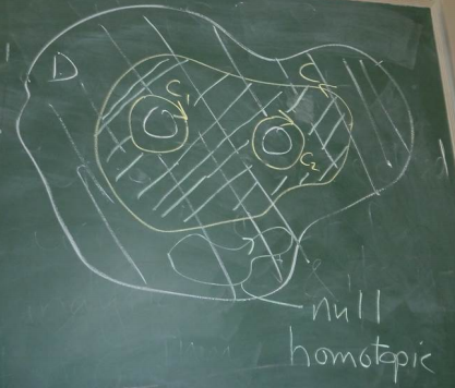
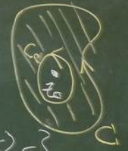
Recall (?) that a domain D is simply connected if for every simple closed contour C in D, it holds that \operatorname{Int}C\subseteq D. Roughly speaking, this means that D has “no holes”. That is, all simply closed contours are null homotopic.

If D is not simply connected, it is multiply connected.

Theorem. If f is analytic on a contour C, as well as on C_1, \ldots, C_n \subset \operatorname{Int}C and on the interior of the domain bordered by C_1, C_2, \ldots, C_n, and C, C_1, \ldots, C_n are all positively oriented, then \int_C f(z)\,dz + \sum_{j=1}^n \int_{C_j}f(z)\,dz = 0. Note that positively oriented means the that while traversing the contour, the region is on your left. This is particularly important for the orientation of C_1, \ldots, C_n.

Visually,

Lecture 21 — Cauchy Integral Formula

Theorem (Cauchy integral formula). Let f be analytic on and inside a simple closed curve C that is positively oriented (interior is to the left of the curve’s direction). Then, if z_0 \in \operatorname{Int}C we have \begin{aligned} f(z_0) &= \frac 1 {2\pi i} \int_C \frac{f(z)}{z-z_0}\,dz, \quad\text{or}\quad 2\pi if(z_0) = \int_C \frac{f(z)}{z-z_0}\,dz. \end{aligned} This is quite an amazing result. Roughly, f is differentiable and we can know the value of f at a point by the integral of any curve around that point.

Proof. Note that the integrand is not analytic on \operatorname{Int}C because it is not defined at z_0. We will “cut out” this discontinuity so we can apply the Cauchy-Goursat theorem. Set C_\rho = \{z(\theta) = z_0 + \rho e^{i\theta}, 0 \le \theta \le 2\pi\} as a curve around our point z_0, for \rho sufficiently small such that \operatorname{Int} C_\rho \subset \operatorname{Int} C.

We have f(z)/(z-z_0) is analytic on \operatorname{Int}C \setminus \operatorname{Int}C_\rho as well as C and C_\rho. We apply Cauchy-Goursat’s extension to multiply connected domains and that gives us \begin{aligned} \int_C \frac{f(z)}{z-z_0}\,dz &= \int_{C_\rho} \frac{f(z)}{z-z_0}\,dz \\ \implies \int_C \frac{f(z)}{z-z_0}\,dz -f(z_0)\int_{C_\rho}\frac{dz}{z-z_0}&= \int_{C_\rho} \frac{f(z)-f(z_0)}{z-z_0}\,dz \end{aligned} From lecture 20, we know that \int_{C_\rho} \frac{dz}{z-z_0} = 2\pi i because C_\rho is a circle centered at z_0 and this holds for any \rho > 0. Since f is analytic at z_0, it is continuous at z_0 so given \epsilon > 0 there exists \delta > 0 such that |f(z) - f(z_0)|<\epsilon for all |z-z_0| < \delta. Choose \rho < \delta and we will have |f(z_0 + \rho e^{i\theta})-f(z_0)|<\epsilon.

Returning to the equations from above, \begin{aligned} \left|\int_C \frac{f(z)}{z-z_0}\,dz -2\pi i\,f(z_0) \right| &\le \int_{C_\rho} \frac{|f(z)-f(z_0)|}{|z-z_0|}\,dz \end{aligned} Note that all points on C_\rho are exactly \rho away from z_0. Thus, 1/|z-z_0| = 1/\rho. Moreover, the integral \int_{C_\rho} |f(z) - f(z_0)|\,dz is bounded by \epsilon \cdot 2\pi \rho by the M-\ell estimate (here, M is \epsilon and \ell is the circumference of a circle with radius \rho). This gives us, \begin{aligned} \int_{C_\rho} \frac{|f(z)-f(z_0)|}{|z-z_0|}\,dz &= \frac 1 \rho \int_{C_\rho} |f(z) - f(z_0)|\,dz \\ &< \frac 1 \rho \epsilon \cdot 2\pi\rho = 2\pi\epsilon \end{aligned} By sending \epsilon \to 0, we can make this arbitrarily small which tells us \begin{aligned} \left|\int_C \frac{f(z)}{z-z_0}\,dz -2\pi i\,f(z_0) \right| = 0 \iff f(z_0) = \frac 1 {2\pi i}\int_C \frac{f(z)}{z-z_0}\,dz, \end{aligned} as required. \square

Lecture 22 — Morera, Liouville Theorem

Recall the Cauchy integral formula: If f is analytic on and inside the simple closed curve C, traversed positively, and z_0 \in \operatorname{Int} C, then f(z_0) = \frac 1 {2\pi i}\int_C \frac{f(z)}{z-z_0}\,dz. Theorem. Under the same conditions, f^{(n)}(z_0) = \frac{n!}{2\pi i}\int_C \frac{f(z)}{(z-z_0)^{n+1}}\,dz. Proof. See exercise 9 of §57 (8 Ed §52). \square

As a result, this tell us that for f = u+iv and f analytic at z_0 = x_0 + iy_0, we know that partials of all orders of u and v exist and are continuous at (x_0, y_0). This is very different from the situation in \mathbb R, where it is very easy to have functions with continuous derivatives but not differentiable. For example, with f(x) = |x|^3, f, f' and f'' are continuous but f'''(0) does not exist.

Note: If f is analytic at z_0, then its derivatives of all orders exist and are analytic at z_0.

Theorem (Morera). Let f be continuous on a domain \Omega. If \int_C f(z)\,dz = 0 for all closed contours C in \Omega, then f is analytic on \Omega.

Proof. By the theorem from lecture 19, f has a primitive F because \int_Cf(Z)\,dz = 0. But then, F' = f exists and is continuous on \Omega by assumption of the theorem. This tell us that F is analytic. Hence, by the note above, f = F' is also analytic. \square

A number of nice results follow from the theorem with f^{(n)}(z_0) above.

Result (I). Let f be analytic in and on C_R(z_0) (curve of a circle of radius R around z_0) and set M_R = \max_{z \in C_R}|f(z)|. Then, \left|f^{(n)}(z_0)\right| \le \frac{n!M_R}{R^n}. This tells us that if we know what the function does on the circle, we can estimate the size of its derivatives at a point. In fact, the closer we get, the worse this estimate becomes because of the division by R^n.

Proof. M_R is well defined by the extreme value theorem. Then, applying the aforementioned theorem, \begin{aligned} \left|f^{(n)}(z_n)\right| = \left|\frac{n!}{2\pi i} \int_{C_R}\frac{f(z)}{(z-z_0)^{n+1}}\,dz\right| &\le \frac{n!}{2\pi}\int_{C_R}\frac{|f(z)|}{|z-z_0|^{n+1}}\,dz \\ &\le \frac{n!M_R}{2\pi R^{n+1}}\int_{C_R}dz \\ &= \frac{n!M_R}{R^n} \end{aligned} Above, note that |z-z_0|=R on this contour, and \int_{C_R}dz is just the arc length of C_R (equal to 2\pi R). \square

As a brief discussion, we have all these powerful results about analytic functions in \mathbb C. However, this hints that being complex differentiable is actually a very restrictive condition.

Result (II – Liouville). If f : \mathbb C \to \mathbb C is bounded and entire (everywhere differentiable), then f is constant.

Proof. Suppose |f| \le M on all of \mathbb C and it is entire. Apply result I for n=1 on C_R(z_0), an arbitrary circle around z_0. The result implies that |f'(z_0)| \le \frac{1!M}R = \frac M R. Letting R \to \infty, we see that f'(z_0) = 0. Since z_0 was arbitrary, we have the result. \square

This is clearly not the case in \mathbb R.

Result (III – Fundamental theorem of algebra). An n-th degree polynomial has exactly n zeros.

Lecture 23 — Conformal Maps, Harmonic Functions

Conformal maps

§112 (8 Ed §101)

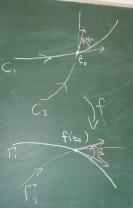
Definition. A conformal map f is a map f : z \mapsto w where f is analytic and f'(z_0) \ne 0. Then locally (near z_0), f preserves angles, orientation, and shape.

In the image below, \Gamma_1 and \Gamma_2 are the images of C_1 and C_2 under f. The angles between them are \alpha and \beta. They intersect at z_0 and f(z_0), respectively. That is, \Gamma_1 = f(C_1) and \Gamma_2=f(C_2). Conformality tells us that \alpha = \beta.

If orientation (i.e. sense, direction) is not necessarily preserved but the angle’s magnitude is, the map is called isogonal.

If instead we had an analytic function with f'(z_0)=0, then z_0 is a critical point of f. This means the angle is not preserved around z_0. However, the angle will be multiplied by m where m is the smallest integer such that f^{(m)}(z_0) \ne 0.

§113 (8 Ed §103)

Conformality means the map is locally 1-to-1 and onto. That is, f has a local inverse. This follows from MATH2400/1’s inverse function theorem. Specifically, it is locally invertible if \det J_f \ne 0. In this case, \begin{aligned} \det J_f = \begin{vmatrix}u_x & u_y \\ v_x & v_y\end{vmatrix} = u_x v_y - u_y v_x = u_x^2 + v_x^2 = |u_x + iv_x|^2 = |f'|^2 \ne 0 \end{aligned} due to f'(z_0) \ne 0 and analyticity of f.

Harmonic functions

We look for a function U : \Omega \to \mathbb R such that \Delta U = 0 \quad\text{(or alternatively, }\nabla^2U=0\text{)}.

Here, \Delta or \nabla^2 is the Laplacian/Laplace operator defined as \Delta U = U_{xx} + U_{yy} or more generally in \mathbb R^n, \Delta = \sum_{j=1}^n U_{jj}. This is used to model many physical situations in “steady state”.

Motivation

Take a region \Omega \subset \mathbb R^2 or \mathbb R^3. Let \Lambda be a “sufficiently smooth subdomain of \Omega”. Some intuition is that an arbitrary point \mathbf x on the \partial \Lambda has an external normal, denoted \boldsymbol{\nu}(\mathbf x) with unit normal \boldsymbol{\nu}'(\mathbf x).

U is the density of something “in equilibrium”, and \mathbf F is the flux density of U in \Omega “in equilibrium”.

This means that along the boundary of \Lambda, \int_{\partial \Lambda} \mathbf F \cdot \boldsymbol{\nu}'\,dS = 0, where dS is the surface measure on \partial \Lambda (i.e. one dimension lower). This means the net in-flow and out-flow are equal. In terms of fluids, this means there are no sources and sinks.

We apply Gauss divergence theorem with the above integral which tells us that \int_{\partial \Lambda} \mathbf F \cdot \boldsymbol{\nu}'\,dS=\int_\Lambda \operatorname{div}\mathbf F\,d\mathbf x = 0 where d\mathbf x = dx\,dy in 2D, etc. Since \Lambda is essentially arbitrary, there holds \operatorname{div}\mathbf F = 0 in \Omega. That is, \sum_{j=1}^n \partial_j F_j = 0 in \Omega.

In many physical situations, \mathbf F = c \nabla U with c usually negative (corresponding to repelling forces). This means that \begin{aligned} \operatorname{div}\mathbf F &= c\operatorname{div}\nabla U = 0 \implies \operatorname{div} \nabla U = \Delta U = 0. \end{aligned}

Lecture 24 — Harmonic Conjugates

Recall from last lecture, conformal maps and Laplacian of harmonic functions.

If U is the concentration of something “in equilibrium”, that implies (somewhat) that \Delta U = 0. There are many solutions to this in general (constants, linear, etc) however we are often interested in boundary conditions.

Can we also study \frac{\partial U}{\partial t} = \alpha \Delta U? As the left hand side approaches 0, the Laplacian approaches 0 and the system approaches steady state. This has many physical applications.

• If U is concentration of a chemical, this is Fick’s law of chemical diffusion.
• If U is temperature, this is Fourier’s law of heat conduction.
• If U is the electric potential, this is Ohm’s law of electrical conduction.

Examples:

• On \mathbb R^2 \setminus \{(0,0)\}, f(x,y) = \ln (\|(x,y)\|) is harmonic.
• On \mathbb R^n \setminus \{\mathbf 0\}, f(\mathbf x) = 1/\|\mathbf x\|^{n-2} is harmonic.

Note that these are radial functions around 0. But how badly do they behave?

Theorem. If f(z) = u(x,y) + iv(x,y) is analytic in \Omega \subseteq \mathbb C, then u and v are harmonic in \Omega.

Proof. Recall that if f is analytic then u and v have continuous partials of all orders and C/R holds. That is, u_x = v_y and u_y = -v_x. We can differentiate these and apply C/R again to get \begin{aligned} u_{xx} &= v_{yx} & u_{xy} &= -v_{xx} \\ u_{yx} &= v_{yy} & u_{yy} &= -v_{yx} \end{aligned} Since partials of all orders are continuous, by Clairaut’s theorem, u_{xy} = u_{yx} and v_{xy} = v_{yx}. Therefore, u_{xx} = v_{yx} = -u_{yy} and similarly for v, so \Delta u = 0 and \Delta v = 0. \square

Definition. If u and v are harmonic and satisfy C/R, then v is called a (not the) harmonic conjugate of u. Note that this is not symmetric.

Theorem. f = u+iv is analytic in \Omega if and only if v is a harmonic conjugate of u.

Proof. (\rightarrow) is done above. (\leftarrow) v is a harmonic conjugate so u and v are both harmonic and u, u_x, u_y, u_{xx}, u_{yy} all exist, are continuous and satisfy C/R throughout \Omega, f is analytic. \square

Example: Suppose v and w are harmonic conjugates of u. This means that u+iv and u+iw are both analytic. Applying C/R, \begin{aligned} u_x &= v_y = w_y, \quad \text{and}\quad u_y = -v_x = -w_x. \end{aligned} Integrating the derivatives of v and w wrt their partial variable, we get v = w + \phi(x) and v = w+\psi(y). Therefore, \phi(x) = \psi(y) which must be a constant. This means v = w+c. \circ

A similar procedure can be used to find a harmonic conjugate of a given harmonic function u.

Example: Find a harmonic conjugate of u(x,y) = y^3 - 3x^2y.

ui s a polynomial function of x and y so has continuous partials of all orders. Moreover, u_{xx}+u_{yy} = 0. Suppose v is a harmonic conjugate of u. C/R tells us u_x = v_y so v_y = -6xy. Integrating this wrt y gives us v = -3xy^2 + \phi(x). Using this in the second part of C/R, \begin{aligned} u_y &= -v_x \\ 3y^2 - 3x^2 &= 3y^2 - \phi'(x) \\ \phi'(x) &= 3x^2\\ \phi(x) &= x^3 + c \end{aligned} So, we can choose c =0 and v(x,y) = -3xy^2+x^3 is a harmonic conjugate of u. Note that in this example, u=\operatorname{Re}f and v=\operatorname{Im} f where f(z) = iz^3.

Lecture 25 — Transformations of Harmonic Functions

Recall harmonic conjugates. That is, v is a harmonic conjugate of u if u and v satisfy C/R.

Remark: v is a harmonic conjugate of u does not imply u is a harmonic conjugate of v.

Example: u = x^2 - y^2 so v = 2xy. Then, u + iv = z^2 is an entire function (analytic everywhere). Therefore, v is a harmonic conjugate of u. However, if u were actually a harmonic conjugate of v, then v + iu would be analytic. We can check with C/R that this function is analytic nowhere.

Remark: Suppose u is harmonic on a simply connected domain \Omega. Then, u has a harmonic conjugate on \Omega. (§115, 8 Ed §104)

Physical problems

§116 (8 Ed §115)

“Physical” configurations are often modelled by solutions of partial differential equations. Generally, we are interested in solving a PDE subject to associated initial/boundary conditions.

For example, \begin{aligned} (D)\begin{cases} \Delta u = 0 & \text{in }\Omega, \\ u|_{\partial \Omega}=\varphi \end{cases} \end{aligned} which means that \Delta u = 0 within \Omega and u = \phi on the boundary. Here, \Omega and \varphi are known and u is unknown. In particular, \varphi : \partial \Omega \to \mathbb R. This (D) is called the Dirichlet problem for Laplace’s equation, a.k.a. the boundary problem of the first kind.

A practical application is a heat equation with an insulated boundary. (D) can be solved by finding a u that minimises \int_\Omega |\nabla u|^2\,d\mathbf x \quad\text{such that}\quad u|_{\partial \Omega} = \varphi. This can be solved by calculus of variations and functional derivatives.

There are also boundary conditions of the second kind, called Neumann boundary conditions. This is (N) \begin{cases} \Delta u = 0 & \text{in }\Omega,\\ \frac{\partial u}{\partial \boldsymbol{\nu}} = \psi & \text{on }\partial \Omega \end{cases} where \boldsymbol{\nu} is the unit normal function on the boundary. Note that \frac{\partial u}{\partial \boldsymbol{\nu}} = \nabla u(\mathbf x)\cdot \boldsymbol{\nu}(\mathbf x). In practice, we often have homogeneous Neumann boundary conditions, i.e. \psi = 0. This is also referred to as no-slip conditions.

Transformations of harmonic functions

Theorem. If f is conformal and h is harmonic in \Lambda, then H is harmonic in \Omega where H(x,y) =h(u(x,y),v(x,y)).

Proof. Messy in general but straightforward when \Lambda is simply connected. See §115 (8 Ed §104). \square

Example: Take h(u,v) = e^{-v}\sin u which is harmonic on the upper half-plane. Define w = z^2 on \Omega, the first quadrant. Thus, w = u+iv where u = x^2 - y^2 and v = 2xy.

Applying this theorem, we know that H(x,y) = e^{-2xy} \sin (x^2-y^2) is harmonic on \Omega. Note that Dirichlet and Neumann boundary conditions are preserved under conformal transformations (more next lecture). \circ

Lecture 26 — Bubbles, Boundary Transformations

We looked at soap film (last year). The key connection is the Neumann boundary conditions. Recall that harmonic functions can be used to minimise some sort of energy function.

In this case, the soap minimises internal potential energy which is done by minimising the surface area of the bubble. This leads to some interesting behaviour for tetrahedral and cubic wire frames with the edges meeting in the middle (as opposed to spanning the face planes).

Transformations

Suppose f is conformal and C is a smooth (infinitely differentiable) arc in \Omega (or on the boundary of \Omega with some care). Let \Gamma = f(C) and H(x,y) = h(u(x,y),v(x,y)).

• If we have Dirichlet boundary conditions on \Gamma (i.e. h(u,v) = \varphi on \Gamma), then H(x,y) = \varphi on C.
• If we have homogeneous Neumann boundary conditions on \Gamma (i.e. \frac{\partial h}{\partial \mathbf n}=0 for any normal \mathbf n to \Gamma), then \frac{\partial H}{\partial \mathbf N}=0 for any normal \mathbf N to C.

Example: In \mathbb C (called the w-plane), the function h(u,v)=v=\operatorname{Im} w is harmonic. In particular, it is harmonic on the horizontal strip \Lambda where -\pi/2 < \operatorname{Im}w<\pi/2. We claim that f : z \mapsto \operatorname{Log}z maps \Omega, the right half-plane, onto \Lambda conformally.

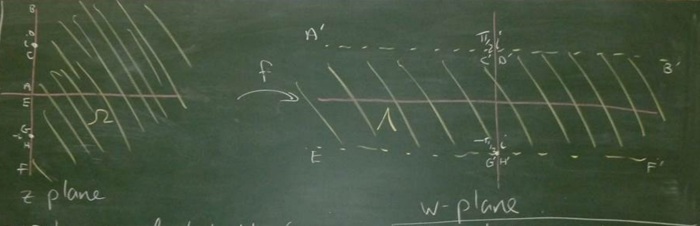
Then, \begin{aligned} z =x+iy\mapsto \operatorname{Log}z &= \ln |z| + i \operatorname{Arg}z \\ &= \underbrace{\ln \sqrt{x^2 +y^2}}_{u} + \underbrace{i\arctan(y/x)}_{iv} \\ \implies H(x,y) &= h(u,v) =\arctan (y/x) \end{aligned} The boundary of \Omega is of the form A = \{0+\delta i : \delta \in \mathbb R\}. Therefore, \begin{aligned} f(A) = \operatorname{Log}A&= \ln |A| + i \operatorname{Arg}A \\ &= \ln |\delta| \pm i\pi/2 \end{aligned} which is exactly the boundary of \Lambda.

Lecture 27 — Heat

Recall that harmonic functions can be mapped to harmonic functions.

Steady-state temperature in a half-plane

§119 (8 Ed §107).

Let \Omega be the upper half-plane. We apply heat to the boundary such that the temperature is 1 between -1 and 1 and 0 everywhere else. We want to find the steady state temperature distribution on \Omega.

Fourier’s law of heat conductions tells us that \begin{aligned} \frac{\partial T}{\partial t} &= \nabla \cdot(-k^2\nabla T) = -k^2\Delta T. \end{aligned} Moreover, steady state tells us that this derivative is 0 so \Delta T = 0.

So, we want to solve \begin{aligned} (D)\begin{cases} \Delta T = 0 & \text{in }\Omega,\\ T(x,0)=\begin{cases} 1 & |x| < 1 \\ 0 & |x| \ge 1 \end{cases} & \text{for }x \in \mathbb R. \end{cases} \end{aligned} Because the temperature being added is 1, the temperature on the plane is bounded between 0 and 1. However, allowing exponentially growing functions (in y) will lead to non-physical solutions.

Note that in \mathbb C (call it the w-plane), h(u,v) = v = \operatorname{Im}w is harmonic. Back to (D), we are looking for a bounded solution with \lim_{y\to\infty}T(x,y)=0 for all x.

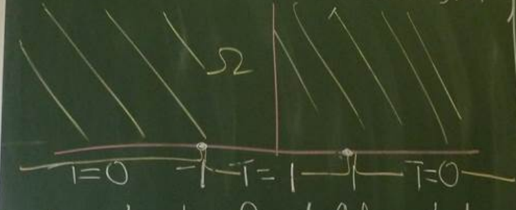
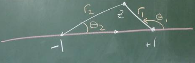
Define \tilde \Omega = \{z : \operatorname{Im}z \ge 0, z \ne \pm 1\}, i.e. \Omega and its boundary excluding the discontinuities. Define \theta_1, \theta_2, r_1, r_2 on \tilde \Omega such that \begin{aligned} z-1 &= r_1 \exp (i\theta_1) \\ z+1 &= r_2 \exp (i\theta_2) \end{aligned} Here, these are defining radial coordinates centred at +1 and -1. r_1, r_2 > 0 and 0 \le \theta_1, \theta_2 \le \pi.

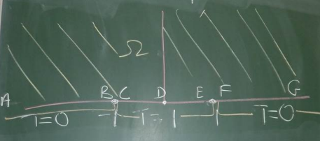
We introduce the transformation \begin{aligned} w = \operatorname{\mathcal {Log}}\frac {z-1}{z+1}, \end{aligned} where \operatorname{\mathcal {Log}} has a branch cut on the negative imaginary axis, so -\pi/2 < \operatorname{\mathcal{Log}}\le 3\pi/2. Then, \begin{aligned} w = \operatorname{\mathcal{Log}}\frac{r_1\exp(i\theta_1)}{r_2\exp(i\theta_2)} = \ln \frac{r_1}{r_2} + i(\theta_1-\theta_2) \end{aligned} We claim that w maps the interior of \Omega onto \Lambda, the horizontal strip 0 < v<\pi. We can look at points along the boundary of \Omega and see where they map to on the boundary of \Lambda.

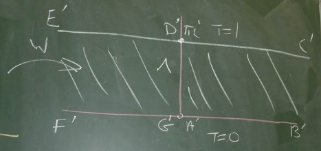
We have transformed our boundary conditions to a problem which can be solved much easier. We just need to find a function satisfying T|_{v=\pi i}=1 and T|_{v=0}=0. Indeed, v/\pi is a bounded harmonic function satisfying these constraints. So, \begin{aligned} w &= \ln \left|\frac{z-1}{z+1}\right| + i \operatorname{\mathcal{Arg}}\frac{z-1}{z+1} \\ \implies v &= \operatorname{\mathcal{Arg}}\left(\frac{z-1}{z+1}\frac{\overline{z+1}}{\overline{z+1}}\right) \\ &= \operatorname{\mathcal{Arg}}\left(\frac{x^2 + y^2 - 1 + 2iy}{(x+1)^2+y^2}\right) \\ &= \arctan\left(\frac{2y}{x^2+y^2-1}\right) \end{aligned} where 0 \le \arctan \le \pi with special care when x^2 + y^2 = 1. The solution is then \frac 1 \pi \arctan \frac{2y}{x^2+y^2-1}. We can check that this is bounded between 0 and 1. This can be visualised using colour or isotherms of the form T(x,y)=c which are circular arcs like x^2 + (y-\cot(\pi c))^2=\csc^2(\pi c).

Lecture 28 — Scale Factor, Poisson’s Integral Formula

Recall that a conformal map preserves angles, orientations and is 1-to-1. However, it can scale points.

Suppose f : z \mapsto w is a conformal map (i.e. analytic and f'(z_0) \ne 0). For z near z_0 with z \ne z_0, \begin{aligned}\frac{|f(z) - f(z_0)|}{|z-z_0|} \approx |f'(z_0)| \quad\implies\quad |f(Z) - f(z_0)| \approx |f'(z_0)|\,|z-z_0|.\end{aligned} Here, |f'(z_0)| is the scaling factor or dilation factor, i.e. the magnitude of the stretching or shrinking effect.

Example: f(z) = z^2 at z_0 = 1+i (here, z = x+iy and w = u+iv). Then, u=x^2-y^2 and v = 2xy.

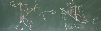
Observe that the tangent lines and angles are preserved under f. The scaling factor is |f'(z_0)| = 2|z_0| = 2\sqrt 2. For a small length near z_0, its length will be scaled by a factor of 2\sqrt2. Thus, \ell' \approx 2 \sqrt 2 \ell and also, \operatorname{Area}(B) \approx (2\sqrt 2)^2 \operatorname{Area}(A). This relationship holds regardless of the curves C_1 and C_2, and for all points z_0.

Poisson’s integral formula

§135 (8 Ed 7§124)

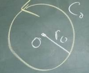
Recall that from Cauchy, if f is analytic in and on C_0, then for z \in \operatorname{Int}C_0, f(z) = \frac1{2\pi i}\int_{C_0}\frac{f(\xi)}{\xi-z}\,d\xi. Recall that for z = re^{i\theta}, r>0, the inverse point to z relative to the circle C_0 is r^*e^{i\theta} with r^* such that r^*r = r_0^2. Also, note that z^* = r^*e^{i\theta}=\frac{r_0^2}re^{i\theta} = \frac{r_0^2}{re^{-i\theta}}=\frac{r_0^2}{\bar z} = \frac{\xi \bar \xi}{\bar z} \quad\text{ for }\xi \in C_0. Now fix z \in \operatorname{Int}C_0 and z \ne 0. Note that \begin{aligned} \int_{C_0} \frac{f(\xi)}{\xi-z^*}\,d\xi=0\quad\text{because}\quad\xi \mapsto\frac{f(\xi)}{\xi-z^*} \end{aligned} is analytic in and on C_0 since z^* \in \operatorname{Ext}C_0 by the Cauchy integral formula. Using this in the above expression, \begin{aligned} f(z) &= \frac 1 {2\pi i} \int_{C_0} \underbrace{\left(\frac 1 {\xi-z}-\frac 1{\xi-z^*}\right)}_{I}f(\xi)\,d\xi \\ I &= \left(\frac \xi {\xi-z} - \frac \xi {\xi - z^*}\right)\frac 1 \xi \\ &= \left(\frac \xi {\xi-z}-\frac 1{1-\bar \xi/\bar z}\right)\frac 1 \xi \\ &= \left(\frac \xi {\xi-z}-\frac{\bar z}{\bar z - \bar \xi}\right)\frac 1 \xi\\ &= \left(\frac{\xi\bar\xi-z\bar z}{|\xi-z|^2} \right)\frac 1 \xi \end{aligned} Recall that z = re^{i\theta}. Put \xi = r_0 e^{i\phi} for 0 \le \phi \le 2\pi. Then, d\xi = r_0ie^{i\phi}\,d\phi. Substituting this into the integrand, \begin{aligned} I &= \frac{r_0^2-r^2}{|\xi-z|^2}\cdot \frac 1 {r_0e^{i\phi}}. \end{aligned} This is mostly in nice radial coordinates except for the |\xi-z| part. Can we rewrite this? Consider the diagram below.

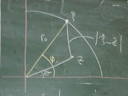
We can appeal to the cosine rule which tells us that |\xi-z|^2 = r_0^2 + r^2 - 2r_0r\cos(\phi-\theta). Plugging this back into f(z), we have \begin{aligned} f(z)=f(re^{i\theta}) &= \frac 1 {2\pi i}\int_0^{2\pi}\frac{r_0^2-r^2}{|\xi-z|^2}\cdot\frac{f(r_0e^{i\phi})r_0ie^{i\phi}}{r_0e^{i\phi}}\,d\phi \\ &= \frac{r_0^2 - r^2}{2\pi}\int_0^{2\pi} \frac{f(r_0e^{i\phi})}{r_0^2 -2r_0r\cos(\phi-\theta)+r^2}\,d\phi \end{aligned}

Recall that the real part of a complex analytic function is harmonic. Taking the real part of the above expression and given “nice enough” \Phi(r_0, \phi) defined on the boundary C_0 of B_{r_0} a (in fact, the) solution of the Dirichlet problem \begin{cases} \Delta u = 0 & \text{in }B_{r_0}, \\ u|_{\partial B_{r_0}} = \Phi(r_0, \phi)& \text{on }\partial B_{r_0}, \end{cases} is given by u(r, \theta) = \frac 1 {2\pi}\int_0^{2\pi}\underbrace{\frac{r_0^2-r^2}{r_0^2-2r_0r\cos(\phi-\theta)+r^2}}_{P(r_0,r,\phi,\theta)}\Phi(r, \phi)\,d\phi. The middle fraction of the integrand is called the Poisson kernel, denoted P(r_0,r,\phi,\theta) and is due to Poisson (1885). This is valid for r=0 too!

Lecture 29 — Sequences and Series

The first part of this lecture was finishing the Poisson integral formula and is written in the previous document.

Complex sequences & series

§60 (8 Ed §55)

Compare this to the situation in \mathbb R. Formally, a sequence is a function f : \mathbb N \to \mathbb C (or \mathbb N _0\to \mathbb C), n \mapsto z_n, written as \{z_n\}.

Definition (Limit). We say \lim_{n \to \infty}z_n = z or “\{z_n\} converges to z” if and only if given \epsilon > 0, there exists N \in \mathbb N such that n > N implies |z_n-z|<\epsilon. As in \mathbb R, this definition does not help us find a limit.

Definition (Series). Formally, \sum_{n=0}^\infty z_n for z_n \in \mathbb C converges as a series if and only if the associated sequence of partial sums \{s_n\} converges as a sequence, where s_n = \sum_{k=0}^n z_k.

A typical question we might ask is does \sum z_n converge?

An easy test that a series does not converge is the n-th term test, if \sum z_n converges, then z_n \to 0 (converse does not hold). Once we know it converges, we know that \sum z_n is just a complex number.

Remark: A sequence \{z_n\} is bounded if there exists M such that |z_n|<M for all n.

Convergent implies that a sequence is bounded (converse does not hold, see \{(-1)^n\}).

Definition (Absolute convergence). We say that \sum z_n converges absolutely if and only if \sum |z_n| converges. Absolute convergence implies convergence (converse does not hold, see \sum (-1)^n/n).

Definition (Remainder). Given \sum_{n=0}^\infty z_n, set s_n=\sum_{k=0}^n z_k as the partial sums. Then, let \rho_n = \sum_{k=n+1}^\infty z_k as the tail or remainder.

Theorem. s_n \to s if and only if \rho_n \to 0.

Example: We claim that \sum_{n=0}^\infty z_n = 1/(1-z)=S for |z| < 1.

Proof. \begin{aligned} s_n &= 1 + z + \cdots + z^n \\ zs_N &= z + z^2 + \cdots + z^{n+1} \\ \implies (1-z)s_n &= 1 - z^{n-1} \\ s_n &= \frac{1-z^{n+1}}{1-z}\\ \implies \rho_n=s-s_n&= \frac {z^{n+1}}{1-z} \end{aligned} Since |z|<1, |\rho_n| \to 0 as n \to \infty which implies that s_n \to s. \square

Remark: As in \mathbb R, we can do simple operations on convergent series:

• If \sum a_n and \sum b_n converge, then \sum (a_n\pm b_n) converges to \sum a_n \pm \sum b_n.
• If \sum a_n converges, then \sum(\lambda a_n) converges to \lambda \sum a_n, for \lambda \in \mathbb C.

Definition (Power series). A power series centred at z_0 is a series of the form \sum_{n=0}^\infty a_n(z-z_0)^n. This series has a radius of convergence. R. That is, it converges absolutely within this radius, diverges outside, and may converge or diverge on the boundary. (These can be checked with the ratio test.)

If R = 0, the series converges only at z_0. If R = \infty, it converges on all of \mathbb C.

Lecture 30 — Taylor Series and Taylor’s Theorem

Theorem (Taylor’s Theorem). Let f be analytic on B_R(z_0). Then, f has a power series representation on B_R(z_0) for |z-z_0|<R as f(z) = \sum_{n=0}^\infty a_n(z-z_0)^n\quad \text{where}\quad a_n = \frac{f^{(n)}(z_0)}{n!}. Note that this is an incredibly powerful statement; unlike \mathbb R, the function is given by the power series. However, the analytic condition is very restrictive.

For the case of z_0=0, this is called the Maclaurin series.

Example: What is the Maclaurin series of f(z) = e^z? f is entire which means that R=\infty. Also, f^{(n)}(0) = e^0=1 for all n. Thus, e^z = \sum_{n=0}^\infty \frac {z^n}{n!}. Proof. Assume z_0 = 0, otherwise translate. Choose z \in B_R, let |z|=r and fix r_0 \in (r, R). Set C = C_{r_0}, positively oriented.

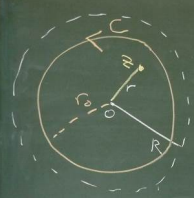
Cauchy integral formula tells us that the value of this analytic function at z is just \begin{aligned} f(z) &= \frac 1 {2\pi i}\int_C \frac{f(\xi)}{\xi-z}\,d\xi. \end{aligned} Looking at the integrand, \begin{aligned} \frac 1 {\xi-z} &= \frac 1 \xi \left(\frac 1 {1-z/\xi}\right) \\ &= \frac 1 \xi \left(\sum_{n=0}^{N-1}(z/\xi)^n + \frac{(z/\xi)^N}{1-z/\xi}\right) \\ &= \sum_{n=0}^{N-1}\frac {z^n}{\xi^{n+1}} + \frac{z^N}{(\xi-z)\xi^N} \end{aligned} The integral becomes \begin{aligned} f(z) &= \frac 1 {2\pi i}\int_C \frac{f(\xi)}{\xi-z}\,d\xi = \sum_{n=0}^{N-1}\frac 1{2\pi i}\int_C \frac{f(\xi)z^n}{\xi^{n+1}}\,d\xi + \underbrace{\frac{z^N}{2\pi i} \int_C \frac{f(\xi)}{(\xi-z)\xi^N}\,d\xi}_{\rho_{N-1}(z)} \end{aligned} We call the rightmost part \rho_{N-1}(z). We can use Cauchy’s integral formula along with the extended Cauchy integral formula (which gives us derivatives), we get f(z) = \sum_{n=0}^{N-1}\frac{f^{(n)}(0)z^n}{n!} + \rho_{N-1}(z).

At this point, we’d like to show that \lim_{N \to \infty}\rho_{N-1}(z) = 0. Note that \xi \in C \implies |\xi| = r_0. Suppose there exists M_N such that we can bound the integrand with \left|\frac{f(\xi)}{(\xi-z)\xi^N}\right| \le M_N \quad \text{on }C. Then, we would be able to say |\rho_{N-1}(z)| \le \frac{r^N}{2\pi}M_N \ell(C) = r_0r^N M_N. To find such an M_N, f is analytic implies |f| is continuous. C is closed and bounded, so extreme value theorem (even just of a single parameter along the curve) implies there exists \mu such that |f| \le \mu on C. Furthermore, |\xi|^N = r_0^N. Using reverse triangle inequality, |\xi-z| \ge \left||\xi|-|z|\right| = r_0-r (note direction of inequality because this is in the denominator).

Putting this all together, M_N = \frac \mu {r_o^N (r_0-r)} suffices for what we want. Then, |\rho_{N-1}(z)| \le r_0r^N M_N = \frac{r_0r^N\mu}{r_0^N(r_0-r)} = \frac{\mu r_0}{r_0-r}\left(\frac r {r_0}\right)^N Therefore, |\rho_{N-1}(z)| \to 0 as N \to \infty because r/r_0 < 1. \square

Remark: In \mathbb R, a Taylor series might converge but fail to converge to the function (see Lecture 16).

To calculate radius of convergence of a power series \sum a_n (z-z_0)^n, we can use the ratio test. First, compute \Lambda = \lim_{n \to \infty} \left|\frac{a_{n+1}}{a_n}\right| \quad \implies \quad R = \frac 1 \Lambda. Conventionally, \Lambda=0 \iff R= \infty and \Lambda = \infty \iff R=0. This is easier because the fraction is the regular ratio test ordering.

Example: f(z) = e^z. For this function, R = \infty because e^z = \sum_{n=0}^\infty \frac {z^n}{n!} \quad \implies\quad \Lambda = \lim_{n \to \infty} \frac{1/(n+1)!}{1/n!} = \lim_{n \to \infty} \frac 1{n+1} = 0. Example: f(z) = z^2 e^{3z} and find the Maclaurin series. Note that f is entire, so \begin{aligned} e^{3z} &= \sum_{n=0}^\infty \frac{3^nz^n}{n!} \\ \implies z^2 e^{3z} &= \sum_{n=0}^\infty \frac{3^nz^{n+2}}{n!} = \sum_{n=2}^{\infty} \frac{3^{n-2}z^n}{(n-2)!} \end{aligned} The last step is because we need a power series to have powers of exactly z^n.

Lecture 31 — Laurent Series, Residues at Poles

Example: Consider the Maclaurin series of f(z) = 1/(1-z). Note that f is analytic for |z| < 1 and indeed, on \mathbb C \setminus \{1\}. Moreover, f^{(n)}(z) = \frac{n!}{(1-z)^{n+1}}, \quad z \ne 1. In particular, f^{(n)}(0) = n!. This tells us that the Taylor series of f at 0 is given by T_{f,0}(z) = \sum_{n=1}^\infty z^n. This has \Lambda = \lim_{n \to \infty}1/1=1 which implies R = 1. Taylor’s theorem implies that T_{f,0} converges to f for |z| < 1.

Some things to note here. This is exactly the geometric series formula, which says \frac 1 {1-z}=\sum_{n=0}^\infty z^n for |z|<1. The series converges “out to the first singularity”, here 1.

Example: Find the Maclaurin series of 1/(2+4z) on \mathbb C \setminus \{-1/2\}. Note that we can manipulate it into the familiar form above. \frac 1 {2+4z} = \frac{1/2}{1+2z} = \frac {1/2}{1-(-2z)}=\frac 1 2 \sum_{n=0}^\infty(-2z)^n = \sum_{n=0}^\infty (-1)^n 2^{n-1}z^n, \quad \text{for }|-2z|<1. Example: f(z) = (1+2z^2)/(z^3+z^5). Some clever algebra tricks lead to f(z) = \frac 1{z^3}\left(\frac{2+2z^2}{1+z^2}-\frac 1 {1+z^2}\right) = \frac 1 {z^3}\left(2 - \frac 1 {1+z^2}\right) which is analytic on \mathbb C \setminus \{0, \pm i\}. Note that this wont converge around 0. For |z|<1, 1/(1+z^2) = \sum_{n=0}^\infty (-1)^n z^{2n}. \begin{aligned} f(z) &= \frac 1 {z^3} (2 - (1 - z^2 + z^4 - \cdots)) = \frac 1 {z^3} + \frac 1 z +- z + z^3 + \cdots. \end{aligned} Although this is not defined at 0, it is still useful. It is almost a power series but has some terms involving negative exponents of z.

Laurent series

By Weierstrass (1841) / Laurent (1843).

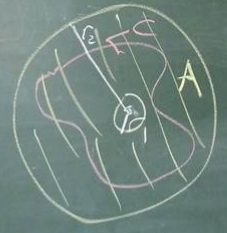
Theorem. Let f be analytic on the open annulus (donut-like shape) A = \{z : r_1 < |z-z_0| < r_2\}, centred at z_0. Let C be a positively oriented, simple, closed curve in A, and let z \in \operatorname{Int}C. Then, f has a series representation, the Laurent series, f(z) = \sum_{n=0}^\infty a_n (z-z_0)^n + \sum_{n=1}^\infty \frac{b_n}{(z-z_0)^n} on A, where \begin{aligned} a_n &= \frac 1 {2\pi i}\int_C \frac{f(\xi)}{(\xi-z_0)^{n+1}}\,d\xi, \qquad b_n = \frac 1 {2\pi i}\int_C \frac{f(\xi)}{(\xi-z_0)^{-n+1}}\,d\xi. \end{aligned} The b_i’s are essentially coefficients of terms of the series with negative exponents (notice the negative power in the integrand the division by (z-z_0)^n).

Alternatively, this can be written as f(z) = \sum_{n=-\infty}^\infty c_n(z-z_0)^n, \quad \text{where }c_n = \frac 1 {2\pi i}\int_C \frac{f(\xi)}{(\xi-z_0)^{n+1}}\,d\xi. In particular with a Laurent series, b_1 = \frac 1 {2\pi i} \int_C \frac{f(\xi)}{(\xi-z_0)^{-1+1}}\,d\xi = \frac 1 {2\pi i}\int_C f(\xi)\,d\xi. This means that if we know the Laurent series, we know the value of this contour integral. This is so important that is has a name, the residue of f at z_0, denoted \operatorname{res}_{z=z_0}f(z). The residue of an analytic function is zero. For example, 1/z has residue 1 at the origin but 0 elsewhere. Here, we are also concerned about the very particular behaviour of the coefficient of z^{-1}.

Notes:

• If f is analytic on and in C, then all the b_i’s are zero.
• The case where r_1 = 0 and r_2 = \infty are both allowed.
• The Taylor and Laurent series are unique. If we have both on an annulus, they coincide. (§72, 8 Ed §66-67).

Example: Find the Laurent series of e^{1/z}. We can just use change of variables with the exponential Taylor series to get e^{1/z}= \sum_{n=0}^\infty \frac 1 {n! z^n} = 1 + \frac 1 z + \frac 1 {2!z^2} for all |z| > 0. Here, there is only one term in the Taylor series part, which is 1. Looking at the coefficient of z^{-1}, we know that \frac 1 {2\pi i}\int_C e^{1/\xi}d\xi = b_1 = 1 for all circles about the origin.

Example 7: Compute I = \int_C \frac{5z-2}{z(z-1)}\,dz where C = 2e^{i\theta} for \theta \in [0, 2\pi]. Note that the integrand f(z) = \frac{5z-2}{z(z-1)} is analytic everywhere except for 0 and 1.

Residues and poles

Definition. We say f : \Omega \to \mathbb C has a singularity at z_0 if

• f is not analytic at z_0, and
• given any \epsilon > 0, there exists z_1 \in B_\epsilon(z_0) such that f is analytic at z_1 (i.e. at some point arbitrarily close to z_0).

In particular, we say f has an isolated singularity at z_0 if f is analytic on B_\epsilon(z_0)\setminus \{z_0\} for some \epsilon > 0.

Examples:

• The function f(z) from Example 7 above has isolated singularities at 0 and 1.

• \operatorname{Log}z has non-isolated singularities on the negative real axis including the origin.

• \sin z / z has an isolated singularity at 0.

• 1/\sin(\pi/z) has isolated singularities at z = 1/k for k \in \mathbb Z and a non-isolated singularity at 0.

Lecture 32 — Cauchy Residue and Product, Singularities

Remark: f(z) = 1/(z-i)^2 is already a Laurent series about i with b_2 = 1 and other coefficients zero.

Cauchy product of series

§73 (8 Ed §67)

Theorem. Suppose f(z) = \sum_{n=0}^\infty a_n z^n and g(z) = \sum_{n=0}^\infty b_nz^n converge. Then, (fg)(z) = \sum_{n=0}^\infty c_nz^n where c_n = \sum_{k=0}^n a_k b_{n-k}.

Example: Consider for |z|<1, \begin{aligned} \frac {e^z}{1+z} = e^z \frac{1}{1-(-z)} &= \left(1 + z + \frac {z^2}{2!} + \cdots\right)\left(1-z+z^2-\cdots\right) \\ &= 1 + (-1+1)z + (1+1/2-1)z^2 + \cdots \\ &= 1 + \frac{z^2}2 + \cdots \end{aligned} Remark: We can take term-by-term derivatives and integrals of series (see §71 or 8 Ed §65).

Cauchy residue theorem

Theorem. Suppose C is a positively oriented simple closed curve and that f is analytic in and on C except at finitely many isolated points \{z_1, z_2, \ldots, z_k\}. Then, \int_C f(z)\,dz = 2\pi i \sum_{j=1}^k \underset{z=z_j}{\operatorname{res}}f(z). Proof. Take disjoint positively oriented circles C_1, \ldots, C_k around each z_1, \ldots, z_k with disjoint interiors, all lying in the interior of C. Then, C, C_1, \ldots, C_k form the boundary of a multiply-connected domain \Omega. Then, f is analytic on \Omega and its boundary, so the Cauchy-Goursat extension implies that \int_C f(z)\,dz = \sum_{j=1}^k \int_{C_j}f(z)\,dz = 2\pi i \sum_{j=1}^k \operatorname{res}_{z=z_j}f(z). \quad \square Example: Apply this to example 7 from last lecture. Note that f is analytic on \mathbb C \setminus \{0,1\} and C is the circle of radius 2 around the origin. I = \int_C \frac{5z-2}{z(z-1)}\,dz. There are two methods we can try. First, look close to zero with 0<|z|<1 to see that \begin{aligned} f(z) = -\frac{1}{1-z}\cdot\frac{5z-2}{z} &= (-1)(1+z+z^2+\cdots)(5-2/z) \\ \implies \underset{z=0}{\operatorname{res}}f(z) &= 2 \end{aligned} Now, we also need a Laurent series around 1 (which is even less fun). We can write \begin{aligned} f(z) &= \frac{5(z-1)+3}{z-1}\cdot\frac{1}{1-(-(z-1))} \\ &= \left(5+\frac3{z-1}\right)(1+(-(z-1))+(-(z-1))^2+\cdots) \\ &\qquad\implies \underset{z=1}{\operatorname{res}}f(z) = 3 \end{aligned} Because the only coefficient of (z-1)^{-1} comes from the 3/(z-1).

Alternatively, we can use partial fractions. Note that f can be decomposed into parts which are analytic on \mathbb C \setminus \{1\} and \mathbb C \setminus \{0\}, respectively. f(z) = \frac{3}{z-1}+\frac 2 z Therefore, this is its own Laurent series around the points 0 and 1. The other fraction is analytic near the other singularity, so does not affect the Laurent series. Therefore, \operatorname{res_{z=0}}f(z) = 2 \qquad \operatorname{res}_{z=1}=3. Note that the expression 3/(z-1) describes, in some sense, the prototypical singularity of a whole family of functions.

Classifying isolated singularities

If z_0 is an isolated singularity of f (i.e. f analytic on a deleted neighbourhood), then there exists R such that f has a Laurent series expansion on B_R(z_0) \setminus \{z_0\} given by f(z) = \sum_{n=0}^\infty a_n(z-z_0)^n + \sum_{n=1}^\infty b_n(z-z_0)^{-n}. There are three cases to consider.

• Case I: If b_n = 0 for all n, then the singularity is removable. Setting f(z_0)=a_0 makes f analytic on all of B_R(z_0).
• Case II: At least one but finitely many of the b_n’s are nonzero. Such a point called a pole. Define m = \max\{n : b_n \ne 0\}. m is the order of the pole and m=1 is a simple pole.
• Case III: Infinitely many of the b_n’s are nonzero. This is an essential singularity.

Lecture 33 — Picard’s Theorem, More Singularities

Recall that isolated singularities fall into three cases. These are points in the complex plane where a function runs into trouble, but is fine in a punctured disk around that point. The three cases are removable, poles, and essential singularities.

These can be defined by, in a deleted ball B_r(z_0) \setminus\{z_0\}, \begin{aligned} &\text{(Case I)} &&\sum_{n \ge 0}a_n(z-z_0)^n \\ &\text{(Case II)} &&\sum_{n \ge -N}a_n(z-z_0)^n, \quad N>1, a_N \ne 0 \\ &\text{(Case III)} && \sum_{n=-\infty}^\infty a_n (z-z_0)^n \end{aligned} Example: f(z) = \sin (z) /z is a function f:\mathbb C^* \to \mathbb C with a singularity at z=0. We can expand \sin into its Taylor series to show that \sin z = \sum_{n=0}\frac{(-1)^nz^{2n+1}}{(2n+1)!} \implies f(z) = \frac 1 z\left(z - \frac {z^3}{3!}+ \cdots\right). The powers of z are all non-negative which means the function is analytic on the deleted ball, so the singularity is removable. If we wanted to define an entire function, we could say \hat f = f on \mathbb C^* and \hat f(0) = a_0=1. Also, the residue is 0.

Example: f(z) = \frac{z^2-1}{z^2-1}\ne 1 which is f : \mathbb C \setminus \{\pm 1\} \to \mathbb C. There are (clearly) two removable singularities at \pm 1. We can’t equate this function to 1, but we could define \hat f : \mathbb C \to \mathbb C with \hat f(z) = 1. This ‘fixes’ the singularity in such a way that you could never tell it was there.

Example: f(z) = 1/z^4 is again defined on \mathbb C^*. There is an isolated singularity at z=0 and this is a pole of order 4.

Example: f(z) = 1/z^4 + 1/z^2 is the same story. The pole is still of order 4; we don’t care about the higher order terms.

Example: f(z) = \sinh (z^2)/z^7, with f : \mathbb C^* \to \mathbb C. Remember that \sinh z = \sum_{n=0}^\infty \frac{z^{2n+1}}{(2n+1)!}. Then, f(z) = \frac 1 {z^7}\sum_{n \ge 0} \frac{z^{4n+2}}{(2n+1)!} = \sum_{n \ge 0}\frac{z^{4n-5}}{(2n+1)!} = \frac 1 {z^5} + \frac 1 z \frac 1 {3!}+\cdots We have a pole of order 5 and the residue is 1/3! in this case.

Example: f(z) = e^{1/z}. In this case, f(z) = \sum_{n=0}^\infty \frac{(1/z)^n}{n!} = 1 + \frac 1 z + \frac 1 {z^2}\frac 1 {2!} + \cdots so we have an essential singularity at z=0 and the residue is 1.

Picard’s theorem

(This is the big version.)

Theorem. Suppose f has an essential singularity at z_0. Let R > 0 be arbitrarily small. Then, on B_R(z_0) \setminus\{z_0\}, the function f attains every value in \mathbb C infinitely often, with the possible exception of one point.

Theorem. If f has a pole of order N at z_0, then in B_r(z_0)\setminus \{z_0\} we can write f(z) = \frac{\phi(z)}{(z-z_0)^N} with \phi analytic in B_r and \phi(z_0)\ne 0. Moreover, \operatorname{res}_{z=z_0} f(z) = \frac{\phi^{(N-1)}(z_0)}{(N-1)!}.

Lecture 34 — Zeros, Poles and Cauchy Principal Value

What is an example of an essential singularity? Consider f(z) = 1/(1-z^{-1}) for z \ne 0. What is the singularity at 0? Observe, f(z) = \frac {1}{1-\frac 1 z}=\frac {z}{z-1} = \frac{-z}{1-z}=-z(1+z+z^2+\cdots) \quad \text{for}\quad0 < |z| < 1. Thus, the singularity is removable because the Laurent series has only non-negative powers. Taking f(0) = 0 extends f to an analytic function on \mathbb C \setminus \{1\}. Moreover, this means the Laurent series is only value out to the singularity at z=1.

Recall that if f has a pole of order n at z_0 and we can write f(z) = \phi(z)/(z-z_0)^n for \phi analytic in B_r(z_0) and \phi(z_0)\ne 0, then \operatorname{Res}_{z=z_0}f= \frac {\phi^{(n-1)}(z_0)}{(n-1)!}. In particular, if z_0 is a simple pole, then \operatorname{Res}_{z=z_0}f=\phi(z_0).

Example: Consider f(z) = (z+i)/(z^2+9). f is analytic on \mathbb C \setminus\{\pm 3i\}, and \pm 3i are isolated singularities. Near z=3i, we can write f(z) = \frac {\phi(z)}{z-3i}\quad \text{where}\quad \phi(z) = \frac {z+i}{z+3i} noting that \phi is analytic and non-zero near 3i. The theorem tells us that \operatorname{Res}_{z=3i}f=\phi(3i)=4i/6i=2/3. We can do the same thing at -3i as well.

Example: f(z) = (z^3+2z)/(z-i)^3. Observe that this is analytic except at i. Near i, f(z) = \frac {\phi(z)}{(z-i)^3} \quad \text{and}\quad \phi(z) = z^3+2z with \phi analytic and \phi(i) \ne 0. Using the same theorem, \operatorname{Res}_{z=i}f={\phi''(i)}/{2!}=3i.

Zeros of functions

§82 (8 Ed §75)

We can generalise the theorem to talk about zeros of functions, because poles are essentially zeros of the denominator.

Lemma. If f is analytic at z_0, then f has a zero of order m at z_0 if \begin{cases} f^{(j)}(z_0)=0& \text{for }j=0, \ldots, m-1, \text{ and} \\ f^{(m)}(z_0)\ne 0. \end{cases} Example: f(z) = (z-i)^4(z-4) has a zero of order 4 at i and a simple zero (i.e. zero of order 1) at 4.

Theorem. f is analytic at z_0 and has a zero of order m at z_0 if and only if f(z) = (z-z_0)^m g(z) where g is analytic and g(z_0)\ne 0.

Zeros & poles

§83 (8 Ed §76)

Theorem. Suppose p and q are analytic at z_0, p(z_0)\ne 0, and q has a zero of order m at z_0. Then, p/q has a pole of order m at z_0.

Example: p(z)=1 and q(z)=z(e^z-1). We know that p/q has an isolated singularity at 0. p is analytic and non-zero everywhere (obviously). We can check that q(0)=0, q'(0)=0, q''(0)=1\ne 0. Thus, p/q has a pole of order 2 at 0.

Theorem. Let p, q be analytic at z_0. If p(z_0)\ne 0 and q(z_0)= 0, then p/q has a simple pole at z_0 and \operatorname{Res}_{z=z_0}\frac p q = \frac {p(z_0)}{q'(z_0)}. Note that there exist higher-order analogues, but they become messy.

Cauchy principal value

The main application of this is contour integrals. In \mathbb R, recall that \begin{aligned} \int_{-\infty}^\infty f(x)\,dx=\lim_{m_1\to\infty}\int_{-m_1}^0 f(x)\,dx+\lim_{m_2\to\infty}\int_0^{m_2}f(x)\,dx. \end{aligned} Note we can replace the split 0 with any fixed c\in \mathbb R. If the limits on the right exist, then we say the integral exists with the given value.

We cannot in general replace the right-hand side with \lim_{m\to\infty}\int_{-m}^mf(x)\,dx. If we do this anyway, it defines the Cauchy principal value (PV) integral.

Example: Let’s look at this in practice. The below improper integral is undefined, because \begin{aligned} \int_{-\infty}^\infty x\,dx &= \lim_{m_1\to\infty}\int_{-m_1}^0x\,dx+\lim_{m_2\to\infty}\int_0^{m_2}x\,dx \\ &= \lim_{m_1\to-\infty}-m_1^2/2+\lim_{m_2\to\infty}m_2^2/2. \end{aligned} However, the principal value is \begin{aligned} \operatorname{PV}\int_{-\infty}^\infty x\,dx = \lim_{m\to\infty}\int_{-m}^m x\,dx=\lim_{m\to\infty}\left[\frac{m^2}2-\frac{m^2}2\right]=0. \end{aligned} Question: When does \operatorname{PV}\int_{-\infty}^\infty f=\int_{-\infty}^\infty f? One case is for even functions or non-negative functions. Specifically, if f is even (so f(x)=f(-x) for all x \in \mathbb R), then \int_0^\infty f(x)\,dx=\frac 1 2 \int_{-\infty}^\infty f(x)\,dx = \frac 1 2 \operatorname{PV} \int_{-\infty}^\infty f(x)\,dx and these integrals converge or diverge together.

Lecture 35 — Cauchy Principal Value Examples

What’s the connection between these integrals and complex analysis? We signed up for the square root of -1 and that’s what we have fun with.

Suppose f is even and “nice” on \mathbb R and we want to evaluate \int_{-\infty}^\infty f(x)\,dx.

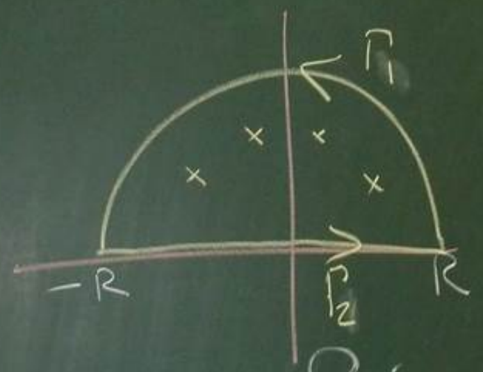
Suppose f is analytic in and on C = \Gamma_1 + \Gamma_2, possibly except for isolated singularities in \operatorname{Int}C. We know that \int_Cf=\int_{\Gamma_1}f+\int_{\Gamma_2}f. Hopefully, we can evaluate the left-hand side with the residue theorem (sum of residues at singularities). Then, if we let R \to \infty, the integral over \Gamma_2 is what we want: \operatorname{PV}\int_{-\infty}^\infty f=\int_{-\infty}^\infty f because we assumed f is even.

It remains to deal with \lim_{R\to\infty}\int_{\Gamma_1}f. Hopefully, we can estimate this to show this goes to zero, for example via M-\ell.

Example: Evaluate I = \int_0^\infty x^2/(x^6+1)\,dx. Note that f(z) = x^2/(x^6+1) is even and continuous. As x \to \pm \infty, f \sim 1/x^4 so I converges by the p-test since p>1. Moreover, the complex function f(z)=z^2/(z^6+1) is analytic on \mathbb C except for 6 zeros of z^6+1, i.e. (-1)^{1/6}.

f is analytic in and on C=\Gamma_1+\Gamma_2 except for the 3 zeros in the upper half-plane. These singularities are z_1=e^{\pi i/6}, z_2=i, and z_3=e^{5\pi i/6}. The residue theorem implies that \int_C f(z)\,dz = 2\pi i\sum_{j=1}^3 \operatorname{Res}_{z=z_j}f. We can see that f has the form p/q and at each z_j, p(z_j)\ne 0, q(z_j)=0, and q'(z_j)\ne 0. Thus, each singularity is a simple pole. From the theorem last lecture of \operatorname{Res}_{z_0}p/q=p(z_0)/q'(z_0), we have \int_Cf(z)\,dz=2\pi i \sum_{j=1}^3 \left.\frac{z^2}{(z^6+1)'}\right|_{z=z_j}=2\pi i\sum_{j=1}^3 \frac{z_j^2}{6z_j^5}=2\pi i\left(\frac 1 {6i}-\frac 1 {6i}+\frac 1 {6i}\right)=\frac \pi 3. Remember that we’re looking for \int_C f=\int_{\Gamma_1}f+\int_{\Gamma_2}f. We’ve got the left-hand side now. As the radius R \to \infty, \int_{\Gamma_2}f \to 2I because we’re looking for the integral from 0 to \infty. Now, we want to show that \int_{\Gamma_1}f \to 0 as R \to \infty. We claim that |\int_{\Gamma_1}f|\le M_R \ell_R where \ell_R is the length of \Gamma_1, which is \pi R. Also, \begin{aligned} M_R &= \max_{z\in\Gamma_1}|f(z)| \le \max_{|z|=R}\left|\frac{z^2}{z^6+1}\right|\le\max_{|z|=R}\frac{|z|^2}{|z|^6-|1|}\le\frac{R^2}{R^6-1} \end{aligned} where the denominator comes from the inverse triangle inequality. Therefore, \lim_{R \to \infty}M_R\ell_R = \lim_{R\to\infty}\frac{\pi R\cdot R^2}{R^6-1}=0. Finally, \int_C f=\int_{\Gamma_1}f+\int_{\Gamma_2}f \implies\frac \pi 3=2I+0\implies I=\frac \pi 6. Example: I=\int_0^\infty \sin x/x\,dx. Firstly, notice that this is an improper integral because the integrand is undefined at 0 and the bound is infinity. Near 0, the integrand approaches 1. Approaching \infty is an absolute pain to estimate (via real analysis).

The good news is \sin x/x is even. If I exists, then I=\frac 1 2\int_{-\infty}^\infty \frac{\sin x}x\,dx=\frac 1 2 \operatorname{PV}\int_{-\infty}^\infty \frac{\sin x}x\,dx. We need to be careful because our theorems don’t work across singularities, despite 0 being a removable singularity. This gives is a 4-part contour.

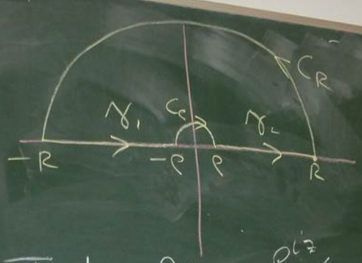
A standard trick when working with trig functions is take an exponential and use the real or imaginary part as needed. Take f(z)=e^{iz}/z which is analytic on \mathbb C_*. Cauchy tells us that the integral across the whole contour is 0. Thus, 0=\int_{\gamma_1+C_\rho+\gamma_2+C_R}f=\int_{\gamma_1}f+\int_{C_\rho}f+\int_{\gamma_2}f+\int_{C_R}f = I_1 + I_2 + I_3 + I_4. Let the integrals of the right-hand side be I_1, \ldots, I_4 respectively. Looking at I_1 and I_3, I_1 = \int_{-R}^{-\rho}\frac{e^{ix}}x\,dx=-\int_\rho^R\frac{e^{-iw}(-w)}{-1}\,dw \quad \text{and} \quad I_3 = \int_\rho^R\frac{e^{ix}}x\,dx. Combining these, I_1+I_3=\int_\rho^R\frac{e^{ix}-e^{-ix}}{x}\,dx=2i\int_\rho^R\frac{\sin x}x\,dx \quad\longrightarrow\quad 2i\int_0^\infty\frac {\sin x}{x}\,dx after taking the limits \rho\to0 and R \to \infty. Therefore, \int_0^\infty \frac {\sin x}{x}\,dx = -\frac 1{2i}\left(\lim_{\rho \downarrow 0}I_2 + \lim_{R \to \infty}I_4 \right) assuming these limits exist. Looking at I_2, we substitute z=\rho e^{i\theta} and \theta : \pi \to 0 (direction) with appropriate change of variables formula. \begin{aligned} I_2 &= \int_{C_\rho}\frac {e^{iz}}{z}\,dz = \int_\pi^0\frac {e^{i\rho e^{i\theta}}}{\rho e^{i\theta}} i\rho e^{i\theta}\,d\theta = -i\int_0^\pi e^{i\rho e^{i\theta}}\,d\theta. \end{aligned} Since |\rho e^{i\theta}| = \rho, the expression e^{i\rho e^{i\theta}}\to 1 as \rho \to 0 uniformly for \theta \in [0,\pi]. From real analysis, this means that the convergence radius \delta is independent of \theta, depending on \epsilon. This means we can write \lim_{\rho \downarrow 0}I_2 = -i\int_0^\pi \lim_{\rho \downarrow 0}\left(e^{i\rho e^{i\theta}}\right)\,d\theta=-i\int_0^\pi d\theta=-i\pi.

Finally, I_4 \to 0 as R \to \infty by Jordan’s lemma (next lecture) because we cannot use M-\ell in the usual way. Therefore, \int_0^\infty \frac {\sin x}{x}\,dx = -\frac 1{2i}\left(\lim_{\rho \downarrow 0}I_2 + \lim_{R \to \infty}I_4 \right)=-\frac 1 {2i }\left[-i\pi+0\right]=\frac\pi 2.

Lecture 36 — Jordan’s Lemma and Rouché’s Theorem

We continued the example of \int_0^\infty \sin x/x\,dx from the previous lecture.

Lemma (Jordan). Suppose f is analytic on the closed upper half plane excluding some disc, \left\{z : \operatorname*{Im}z\ge 0\right\}\cap \left\{z : |z| \ge R_0\right\}, which satisfies |f(z)| \le M/R^\beta for some M, \beta > 0 on the outside arc of \Gamma_R = \left\{Re^{i\theta} : R > R_0, 0 \le \theta \le \pi\right\}. Then, for all \alpha > 0, \lim_{R \to \infty}\int_{\Gamma_R}e^{i\alpha z}f(z)\,dz = 0. Proof. Fairly straightforward apart from one estimate. \square

Argument principle & Rouché’s theorem

§93–94 (8 Ed §86–87) – Rouche’s Theorem

The argument principle says if f is analytic in and on C, a simple closed curve, except possibly for poles inside C, then the rate of change of the argument along the curve is \Delta_C \arg f=2\pi(z\cdot p), where z is the number of zeros inside C counting multiplicity, and p is the number of poles counting sum of orders.

Theorem (Rouché’s theorem). Let f and g be analytic in and on a simple closed curve C (orientation irrelevant). Suppose |g(z)| < |f(z)| for all z on this curve. Then, f and f+g have the same number of zeros (counting multiplicity) inside C.

For example, (z-i)^2(z+i)^3 has 5 zeros counting multiplicity. Make sure to check conditions before applying theorems.

Example: How many zeros of h(z) = z^7-4z^3-1 lie inside the unit circle? Let f(z) = -4z^3 and g(z) = z^7+z-1, noting that both are polynomials and entire. In general for picking f and g with an annulus, take the larger power outside the annulus. This case is a bit more special. First, we have |f|=4 on C and by the triangle inequality, |g(z)| \le |z^7| + |z| + |-1| =3< 4=|f(z)|. Because |g| < |f| on C, Rouché’s theorem implies that f and f+g=h have the same number of zeros inside C, namely 3 because f has a 3-fold zero at 0.

Lecture 37 — Additional

Proof of Jordan’s lemma

Lemma (Jordan). Suppose f is analytic on the closed upper half plane excluding some disc, \left\{z : \operatorname*{Im}z\ge 0\right\}\cap \left\{z : |z| \ge R_0\right\}, which satisfies |f(z)| \le M/R^\beta for some M, \beta > 0 on the outside region \Gamma_R = \left\{Re^{i\theta} : R > R_0, 0 \le \theta \le \pi\right\}. Then, for all \alpha > 0, \lim_{R \to \infty}\int_{\Gamma_R}e^{i\alpha z}f(z)\,dz = 0. Proof. On \Gamma_R, we have z=Re^{i\theta} and dz=iRe^{i\theta}. Substituting in, \begin{aligned} \left|\,\int_{\Gamma_R}e^{i\alpha z}f(z)\,dz\, \right|= R\left|\, \int_0^\pi e^{i\alpha R e^{i\theta}}f(Re^{i\theta})\,d\theta\, \right| &\le R\int_0^\pi \left| e^{i\alpha Re^{i\theta}}f(Re^{i\theta})\right|\,d\theta. \end{aligned} Expanding e^{i\theta} in the inner exponent and taking the modulus gives us \begin{aligned} =R\int_0^\pi \left| e^{i\alpha (R\cos \theta + iR\sin \theta)}f(Re^{i\theta}) \right|\,d\theta = R\int_0^\pi e^{-\alpha R \sin \theta} \left|f(Re^{i\theta}) \right|\,d\theta. \end{aligned} Now we use the bound assumption on f and symmetry of the integrand, \le \frac M{R^{\beta-1}} \int_0^\pi e^{-\alpha R \sin \theta}\,d\theta = \frac {2M}{R^{\beta-1}}\int_0^{\pi/2}e^{-\alpha R\sin \theta}\,d\theta. Note that \sin \theta \ge 2\theta / \pi for 0 \le \theta \le \pi/2 (can be proven via simple calculus). Using this, we have \begin{aligned} \frac {2M}{R^{\beta-1}}\int_0^{\pi/2}e^{-\alpha R\sin \theta}\,d\theta &\le \frac {2M}{R^{\beta-1}}\int_0^{\pi/2}e^{-2\alpha R\theta/\pi}\,d\theta = \frac {2M}{R^{\beta-1}}\frac {\pi}{2\alpha R}\left( 1 - e^{-\alpha R} \right) = \frac {M\pi}{\alpha R^\beta}\left(1-e^{\alpha R}\right) \end{aligned} which we can see goes to 0 as R \to \infty. \square

Trig substitutions in integrals

To solve integrals of the form \int_0^{2\pi }f(\sin t, \cos t)\,dt we can try the substitutions z=\cos t + i \sin t, \quad z^{-1}=\cos t-i \sin t with the motivation being z=e^{it} for 0 \le t \le 2\pi. Then we just need to integrate around the unit circle. This gives us \begin{gathered} \cos t = \frac 1 2 \left(z+z^{-1}\right)\quad \text{and}\quad \sin t=\frac 1 {2i}\left( z - z^{-1} \right) \end{gathered} which implies that dz=(-\sin t + i \cos t)\,dt=iz\,dt. Example: Find I = \int_0^{2\pi}1/(2+\cos t)\,dt. Write z=e^{it} and using the substitution above, dt=\frac {dt}{iz} \quad \text{and}\quad\cos t = \frac 1 2 \left( z+z^{-1} \right). For C = \left\{ e^{it}, 0 \le t \le 2\pi \right\}, we have \begin{aligned} I = \int_C \frac {1/(iz)}{2+1/2\left( z+z^{-1} \right)}\,dz = -i\int_C \frac {dz}{2z+1/2\left( z^2+1 \right)} =-2i\int_C\frac {dz}{z^2+4z+1}. \end{aligned} To evaluate the last integral, note that the integrand is analytic except for zeros of the denominator, -2\pm \sqrt 3. Only -2+\sqrt 3 lies inside C, so by residue theorem I = (-2i)2\pi i \operatorname*{Res}_{z=-2+\sqrt 3}\frac {1}{z^2+4z+1}=\operatorname*{Res}_{z=-2+\sqrt 3}\frac {1/(z-(-2-\sqrt 3))}{z-(-2+\sqrt 3)}. The numerator is analytic and non-zero near -2+\sqrt 3 so the integrand has a simple pole at -2+\sqrt 3. The residue is calculated by \operatorname*{Res}_{z=-2+\sqrt 3}\frac {1}{z^2 + 4z+1}=\phi(-2+\sqrt 3)=\frac {1}{2\sqrt 3} and hence, I = (-2i)2\pi i /(2\sqrt 3)=2\pi / \sqrt 3.

Laurent series of 1/\sinh z

We will try to calculate the Laurent series of 1/\sinh z at 0. This has singularities where \sinh z=0 which is exactly for z=n\pi i, n \in \mathbb Z. Thus, 1/\sinh z has a Laurent series on 0<|z|<\pi. Then, writing out the series, \begin{aligned} \frac {1}{\sinh z} &= \frac {1}{z + z^3/3! + z^5/5! + \cdots} = \frac 1 z \frac {1}{1+z^2/3! + z^4/5! + \cdots}. \end{aligned} For |z^2/3! + z^4/5! + \cdots|<1, we can use the geometric series formula as long as |z| is sufficiently small. \frac 1 {\sinh z} = \frac 1 z \left[ 1 - \left(\frac{z^2}{3!} + \frac{z^4}{5!} + \cdots\right) + \left(\frac{z^2}{3!} + \frac{z^4}{5!} + \cdots\right)^2 - \cdots \right] In particular, there is a pole of order 1 at 0 with \operatorname*{Res}_{z=0}\frac {1}{\sinh z}=1.

Laurent series of \cot z/z^2

We start with \cot z = \cos z / \sin z and the usual Taylor series of \sin and \cos. \begin{aligned} g(z) = \frac {\cot z}{z^2} = \frac 1 {z^2}\frac {\cos z}{\sin z} &=\frac {1} {z^2}\left( \frac {\sum_{n=0}^\infty (-1)^nz^{2n}/(2n)!}{\sum_{n=0}^\infty (-1)^nz^{2n+1}/(2n+1)!} \right) \\ &=\frac {1}{z^2}\frac {\left(1-z^2/2! + z^4/4! - \cdots\right)} {\left(z-z^3/3!+z^5/5!+\cdots\right)} \\ &= \frac {1}{z^3} \frac {\left(1-z^2/2! + z^4/4! - \cdots\right)} {\left(1-z^2/3!+z^4/5!+\cdots\right)} \\ \end{aligned} Above, we expanded the power series of \sin and \cos, then factored a z out of the denominator with the goal of using the geometric series formula. Continuing, \begin{aligned} \frac {1}{z^3} \frac {\left(1-z^2/2! + z^4/4! - \cdots\right)} {\left(1-z^2/3!/+z^4/5!+\cdots\right)} &= \frac {1}{z^3} \frac {\left(1-z^2/2! + z^4/4! - \cdots\right)} {1-(z^2/3!+z^4/5!+\cdots)}. \end{aligned} The tail of the denominator series converges (why?) and has modulus less than 1 (really?) and so we can write this as a geometric series. Expanding a few terms is sufficient to determine the residue. \begin{aligned} g(z)&=\frac {1}{z^3} \left(1-z^2/2! + z^4/4! - \cdots\right) \sum_{n=0}^\infty (z^2/3!+z^4/5!+\cdots)^n \\ &= \frac {1}{z^3} \Big(1-z^2/2! + z^4/4! - \cdots\Big) \Big(1 + (z^2/3!+\cdots) + (z^2/3!+\cdots)^2+\cdots\Big)\\ &= \frac {1}{z^3}\left(1 + \left( \frac {1}{3!}-\frac {1}{2!} \right)z^2 + \cdots\right) \end{aligned} Looking at the fractions, 1/6-1/2=-1/3 so the residue at 0 is -1/3. Anything more than this is going to be very hard.