Recall that harmonic functions can be mapped to harmonic functions.
§119 (8 Ed §107).
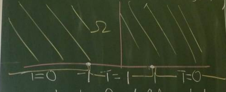
Let \Omega be the upper half-plane. We apply heat to the boundary such that the temperature is 1 between -1 and 1 and 0 everywhere else. We want to find the steady state temperature distribution on \Omega.
Fourier’s law of heat conductions tells us that \begin{aligned} \frac{\partial T}{\partial t} &= \nabla \cdot(-k^2\nabla T) = -k^2\Delta T. \end{aligned} Moreover, steady state tells us that this derivative is 0 so \Delta T = 0.
So, we want to solve \begin{aligned} (D)\begin{cases} \Delta T = 0 & \text{in }\Omega,\\ T(x,0)=\begin{cases} 1 & |x| < 1 \\ 0 & |x| \ge 1 \end{cases} & \text{for }x \in \mathbb R. \end{cases} \end{aligned} Because the temperature being added is 1, the temperature on the plane is bounded between 0 and 1. However, allowing exponentially growing functions (in y) will lead to non-physical solutions.
Note that in \mathbb C (call it the w-plane), h(u,v) = v = \operatorname{Im}w is harmonic. Back to (D), we are looking for a bounded solution with \lim_{y\to\infty}T(x,y)=0 for all x.
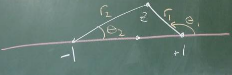
Define \tilde \Omega = \{z : \operatorname{Im}z \ge 0, z \ne \pm 1\}, i.e. \Omega and its boundary excluding the discontinuities. Define \theta_1, \theta_2, r_1, r_2 on \tilde \Omega such that \begin{aligned} z-1 &= r_1 \exp (i\theta_1) \\ z+1 &= r_2 \exp (i\theta_2) \end{aligned} Here, these are defining radial coordinates centred at +1 and -1. r_1, r_2 > 0 and 0 \le \theta_1, \theta_2 \le \pi.
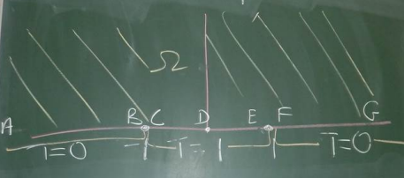
We introduce the transformation \begin{aligned} w = \operatorname{\mathcal {Log}}\frac {z-1}{z+1}, \end{aligned} where \operatorname{\mathcal {Log}} has a branch cut on the negative imaginary axis, so -\pi/2 < \operatorname{\mathcal{Log}}\le 3\pi/2. Then, \begin{aligned} w = \operatorname{\mathcal{Log}}\frac{r_1\exp(i\theta_1)}{r_2\exp(i\theta_2)} = \ln \frac{r_1}{r_2} + i(\theta_1-\theta_2) \end{aligned} We claim that w maps the interior of \Omega onto \Lambda, the horizontal strip 0 < v<\pi. We can look at points along the boundary of \Omega and see where they map to on the boundary of \Lambda.
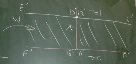
We have transformed our boundary conditions to a problem which can be solved much easier. We just need to find a function satisfying T|_{v=\pi i}=1 and T|_{v=0}=0. Indeed, v/\pi is a bounded harmonic function satisfying these constraints. So, \begin{aligned} w &= \ln \left|\frac{z-1}{z+1}\right| + i \operatorname{\mathcal{Arg}}\frac{z-1}{z+1} \\ \implies v &= \operatorname{\mathcal{Arg}}\left(\frac{z-1}{z+1}\frac{\overline{z+1}}{\overline{z+1}}\right) \\ &= \operatorname{\mathcal{Arg}}\left(\frac{x^2 + y^2 - 1 + 2iy}{(x+1)^2+y^2}\right) \\ &= \arctan\left(\frac{2y}{x^2+y^2-1}\right) \end{aligned} where 0 \le \arctan \le \pi with special care when x^2 + y^2 = 1. The solution is then \frac 1 \pi \arctan \frac{2y}{x^2+y^2-1}. We can check that this is bounded between 0 and 1. This can be visualised using colour or isotherms of the form T(x,y)=c which are circular arcs like x^2 + (y-\cot(\pi c))^2=\csc^2(\pi c).