Lecture 35 — Cauchy Principal Value Examples

What’s the connection between these integrals and complex analysis? We signed up for the square root of $-1$ and that’s what we have fun with.

Suppose $f$ is even and “nice” on $\mathbb R$ and we want to evaluate $\int_{-\infty}^\infty f(x)\,dx$.

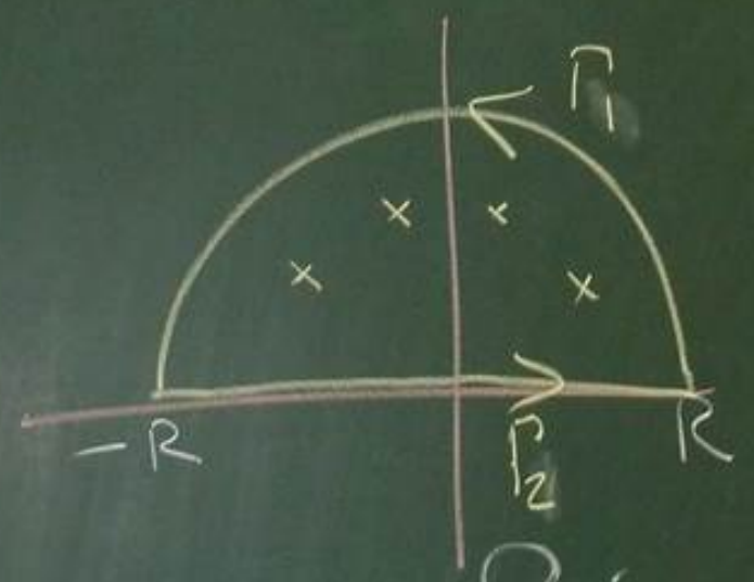
Suppose $f$ is analytic in and on $C = \Gamma_1 + \Gamma_2$, possibly except for isolated singularities in $\operatorname{Int}C$. We know that $\int_Cf=\int_{\Gamma_1}f+\int_{\Gamma_2}f.$ Hopefully, we can evaluate the left-hand side with the residue theorem (sum of residues at singularities). Then, if we let $R \to \infty$, the integral over $\Gamma_2$ is what we want: $\operatorname{PV}\int_{-\infty}^\infty f=\int_{-\infty}^\infty f$ because we assumed $f$ is even.

It remains to deal with $\lim_{R\to\infty}\int_{\Gamma_1}f$. Hopefully, we can estimate this to show this goes to zero, for example via $M$-$\ell$.

Example: Evaluate $I = \int_0^\infty x^2/(x^6+1)\,dx$. Note that $f(z) = x^2/(x^6+1)$ is even and continuous. As $x \to \pm \infty$, $f \sim 1/x^4$ so $I$ converges by the $p$-test since $p>1$. Moreover, the complex function $f(z)=z^2/(z^6+1)$ is analytic on $\mathbb C$ except for 6 zeros of $z^6+1$, i.e. $(-1)^{1/6}$.

$f$ is analytic in and on $C=\Gamma_1+\Gamma_2$ except for the 3 zeros in the upper half-plane. These singularities are $z_1=e^{\pi i/6}$, $z_2=i$, and $z_3=e^{5\pi i/6}$. The residue theorem implies that $\int_C f(z)\,dz = 2\pi i\sum_{j=1}^3 \operatorname{Res}_{z=z_j}f.$ We can see that $f$ has the form $p/q$ and at each $z_j$, $p(z_j)\ne 0$, $q(z_j)=0$, and $q'(z_j)\ne 0$. Thus, each singularity is a simple pole. From the theorem last lecture of $\operatorname{Res}_{z_0}p/q=p(z_0)/q'(z_0)$, we have $\int_Cf(z)\,dz=2\pi i \sum_{j=1}^3 \left.\frac{z^2}{(z^6+1)'}\right|_{z=z_j}=2\pi i\sum_{j=1}^3 \frac{z_j^2}{6z_j^5}=2\pi i\left(\frac 1 {6i}-\frac 1 {6i}+\frac 1 {6i}\right)=\frac \pi 3.$ Remember that we’re looking for $\int_C f=\int_{\Gamma_1}f+\int_{\Gamma_2}f$. We’ve got the left-hand side now. As the radius $R \to \infty$, $\int_{\Gamma_2}f \to 2I$ because we’re looking for the integral from $0$ to $\infty$. Now, we want to show that $\int_{\Gamma_1}f \to 0$ as $R \to \infty$. We claim that $|\int_{\Gamma_1}f|\le M_R \ell_R$ where $\ell_R$ is the length of $\Gamma_1$, which is $\pi R$. Also, $\begin{aligned} M_R &= \max_{z\in\Gamma_1}|f(z)| \le \max_{|z|=R}\left|\frac{z^2}{z^6+1}\right|\le\max_{|z|=R}\frac{|z|^2}{|z|^6-|1|}\le\frac{R^2}{R^6-1} \end{aligned}$ where the denominator comes from the inverse triangle inequality. Therefore, $\lim_{R \to \infty}M_R\ell_R = \lim_{R\to\infty}\frac{\pi R\cdot R^2}{R^6-1}=0.$ Finally, $\int_C f=\int_{\Gamma_1}f+\int_{\Gamma_2}f \implies\frac \pi 3=2I+0\implies I=\frac \pi 6.$ Example: $I=\int_0^\infty \sin x/x\,dx$. Firstly, notice that this is an improper integral because the integrand is undefined at 0 and the bound is infinity. Near $0$, the integrand approaches $1$. Approaching $\infty$ is an absolute pain to estimate (via real analysis).

The good news is $\sin x/x$ is even. If $I$ exists, then $I=\frac 1 2\int_{-\infty}^\infty \frac{\sin x}x\,dx=\frac 1 2 \operatorname{PV}\int_{-\infty}^\infty \frac{\sin x}x\,dx.$ We need to be careful because our theorems don’t work across singularities, despite $0$ being a removable singularity. This gives is a 4-part contour.

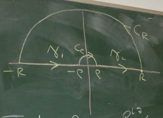
A standard trick when working with trig functions is take an exponential and use the real or imaginary part as needed. Take $f(z)=e^{iz}/z$ which is analytic on $\mathbb C_*$. Cauchy tells us that the integral across the whole contour is 0. Thus, $0=\int_{\gamma_1+C_\rho+\gamma_2+C_R}f=\int_{\gamma_1}f+\int_{C_\rho}f+\int_{\gamma_2}f+\int_{C_R}f = I_1 + I_2 + I_3 + I_4.$ Let the integrals of the right-hand side be $I_1, \ldots, I_4$ respectively. Looking at $I_1$ and $I_3$, $I_1 = \int_{-R}^{-\rho}\frac{e^{ix}}x\,dx=-\int_\rho^R\frac{e^{-iw}(-w)}{-1}\,dw \quad \text{and} \quad I_3 = \int_\rho^R\frac{e^{ix}}x\,dx.$ Combining these, $I_1+I_3=\int_\rho^R\frac{e^{ix}-e^{-ix}}{x}\,dx=2i\int_\rho^R\frac{\sin x}x\,dx \quad\longrightarrow\quad 2i\int_0^\infty\frac {\sin x}{x}\,dx$ after taking the limits $\rho\to0$ and $R \to \infty$. Therefore, $\int_0^\infty \frac {\sin x}{x}\,dx = -\frac 1{2i}\left(\lim_{\rho \downarrow 0}I_2 + \lim_{R \to \infty}I_4 \right)$ assuming these limits exist. Looking at $I_2$, we substitute $z=\rho e^{i\theta}$ and $\theta : \pi \to 0$ (direction) with appropriate change of variables formula. $\begin{aligned} I_2 &= \int_{C_\rho}\frac {e^{iz}}{z}\,dz = \int_\pi^0\frac {e^{i\rho e^{i\theta}}}{\rho e^{i\theta}} i\rho e^{i\theta}\,d\theta = -i\int_0^\pi e^{i\rho e^{i\theta}}\,d\theta. \end{aligned}$ Since $|\rho e^{i\theta}| = \rho$, the expression $e^{i\rho e^{i\theta}}\to 1$ as $\rho \to 0$ uniformly for $\theta \in [0,\pi]$. From real analysis, this means that the convergence radius $\delta$ is independent of $\theta$, depending on $\epsilon$. This means we can write $\lim_{\rho \downarrow 0}I_2 = -i\int_0^\pi \lim_{\rho \downarrow 0}\left(e^{i\rho e^{i\theta}}\right)\,d\theta=-i\int_0^\pi d\theta=-i\pi.$

Finally, $I_4 \to 0$ as $R \to \infty$ by Jordan’s lemma (next lecture) because we cannot use $M$-$\ell$ in the usual way. Therefore, $\int_0^\infty \frac {\sin x}{x}\,dx = -\frac 1{2i}\left(\lim_{\rho \downarrow 0}I_2 + \lim_{R \to \infty}I_4 \right)=-\frac 1 {2i }\left[-i\pi+0\right]=\frac\pi 2.$